
OCR Specification focus:
‘On velocity–time graphs, acceleration equals gradient and displacement equals area under the graph.’
Velocity–time graphs are a fundamental visual tool in kinematics, representing how an object’s velocity changes with time. Understanding how to interpret their gradients and areas allows physicists to determine acceleration and displacement, providing a complete description of motion. These graphs form the bridge between the graphical interpretation of motion and the mathematical use of kinematic equations, a core competency in OCR A-Level Physics.
Understanding Velocity–Time Graphs
A velocity–time graph (v–t graph) plots velocity on the vertical axis against time on the horizontal axis. Each point on the graph represents the instantaneous velocity of an object at a given moment. By examining the shape and slope of the graph, one can extract key motion characteristics such as whether the object is stationary, moving uniformly, or accelerating.
Different sections of a v–t graph provide distinct insights:
A horizontal line indicates constant velocity (zero acceleration).
A sloping line shows uniform acceleration or deceleration, depending on the slope’s direction.
A curved line represents non-uniform acceleration, where acceleration changes with time.
Velocity–time graph: A graphical representation showing how the velocity of an object varies with time, where the gradient gives acceleration and the area under the line gives displacement.
Velocity–time graphs can depict motion in one dimension, where positive velocity indicates movement in one direction (e.g., forward) and negative velocity indicates motion in the opposite direction (e.g., backward). The sign convention is vital in analysing situations involving reversal of motion, such as an object thrown upwards and then returning to its starting point.
Gradients and Acceleration
The gradient (or slope) of a velocity–time graph indicates the rate of change of velocity, which corresponds to acceleration.
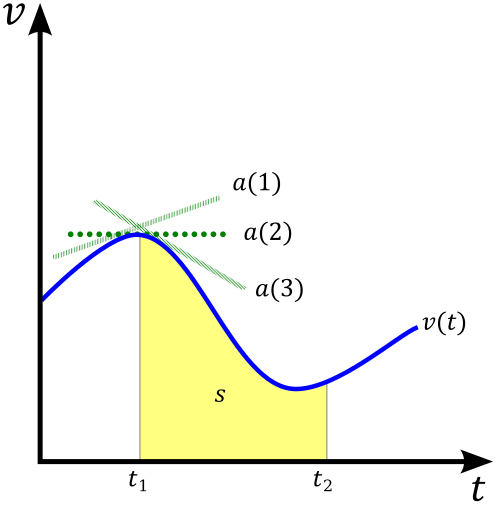
Example velocity–time graph showing how acceleration equals the gradient at any point and displacement equals the area under the curve over a time interval. The layout supports both constant and changing gradients. This directly underpins graphical extraction of motion quantities from v–t data. Source.
Acceleration: The rate of change of velocity with respect to time.
EQUATION
—-----------------------------------------------------------------
Acceleration (a) = Δv / Δt
Δv = Change in velocity (m s⁻¹)
Δt = Time interval (s)
—-----------------------------------------------------------------
A positive gradient represents acceleration (velocity increasing with time), while a negative gradient represents deceleration (velocity decreasing with time). If the graph shows a constant gradient, the acceleration is uniform; if the gradient varies, the acceleration is non-uniform.
In cases where the graph is curved, the instantaneous acceleration at any point can be determined by finding the gradient of the tangent to the curve at that point. This process is central in experimental motion analysis using recorded data.
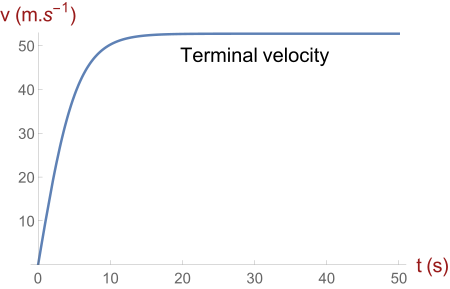
Velocity–time graph for a skydiver showing a rapid rise in speed that levels off at terminal velocity, illustrating non-uniform acceleration. The slope of a tangent gives the instantaneous acceleration at each moment. Extra physical context (air resistance and terminal speed) is included but the graph remains a standard v–t curve. Source.
Gradient Interpretation Examples
Zero gradient → constant velocity (no acceleration).
Steep positive gradient → large, uniform acceleration.
Steep negative gradient → rapid deceleration.
Curved gradient → acceleration changing over time (non-uniform).
These interpretations allow students to qualitatively describe motion even before quantitative analysis begins.
Areas and Displacement
The area under a velocity–time graph represents the displacement of an object during a given time interval. Displacement, a vector quantity, depends on both magnitude and direction, and its sign indicates direction of motion.
Displacement: The vector distance moved by an object in a specific direction from its initial to final position.
EQUATION
—-----------------------------------------------------------------
Displacement (s) = Area under velocity–time graph
—-----------------------------------------------------------------
This relationship holds because multiplying velocity (m s⁻¹) by time (s) yields distance (m). For uniformly accelerating motion, the graph forms simple geometric shapes—such as rectangles, triangles, or trapezia—allowing straightforward calculation of areas. When the graph includes irregular or curved sections, the area can be estimated by dividing it into smaller shapes or by numerical integration methods.
In cases where the velocity becomes negative, areas below the time axis represent displacement in the opposite direction. The net displacement is therefore the algebraic sum of positive and negative areas. The total distance travelled, however, equals the sum of the magnitudes of all areas, ignoring sign.
Area Calculation Summary
Uniform velocity → area is a rectangle (s = v × t).
Uniform acceleration from rest → area is a triangle (s = ½ v t).
Non-zero initial velocity with acceleration → area is a trapezium (s = ½ (u + v) t).
These geometric interpretations directly connect graphical analysis to the standard SUVAT equations of motion.
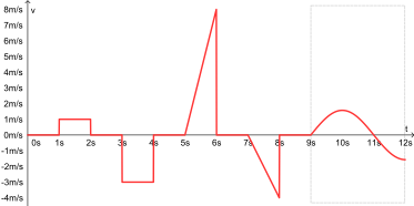
Set of velocity–time curves illustrating constant velocity (horizontal), uniform acceleration/deceleration (straight sloped lines), and non-uniform acceleration (curves). The figure also makes the sign of velocity clear when the graph lies above or below the time axis. Use it to link visual features directly to changes in acceleration. Source.
Physical Meaning and Real-World Application
Interpreting gradients and areas on velocity–time graphs allows scientists to reconstruct an object’s motion entirely from graphical data. For instance:
Measuring the gradient at different points reveals how forces influence acceleration, by linking to Newton’s Second Law (F = ma).
The area reveals total displacement, vital in navigation, trajectory prediction, or transport safety analysis.
In experimental contexts, data-loggers, motion sensors, or video tracking systems capture velocity data over time. Software then generates velocity–time graphs, from which gradients and areas are computed automatically to obtain accurate values of acceleration and displacement. These methods enhance precision beyond what manual measurements allow.
Practical Interpretation Notes
Ensure the velocity scale is correct; any inconsistency leads to proportional error in both gradient and area.
Always check units—velocity in m s⁻¹ and time in seconds ensures displacement in metres.
When analysing non-linear graphs, divide them into smaller intervals where linear approximation is reasonable for estimating areas or gradients.
Understanding how to link these graphical relationships underpins deeper kinematic reasoning in both theoretical and experimental physics. Mastery of the concept that acceleration equals gradient and displacement equals area is essential for interpreting motion, validating equations, and applying models of linear motion across a wide range of physical situations.
Practice Questions
Question 1 (2 marks)
A car’s velocity–time graph shows a straight line rising uniformly from 0 m s⁻¹ to 20 m s⁻¹ over 5.0 s.
(a) Calculate the car’s acceleration.
(b) State what the area under the graph represents.
Mark scheme:
(a)
Acceleration = change in velocity / time = (20 − 0) / 5 = 4.0 m s⁻² (1 mark)
(b)Area under graph represents the displacement of the car (1 mark)
Question 2 (5 marks)
A cyclist starts from rest and accelerates uniformly for 6.0 s until reaching a velocity of 12 m s⁻¹. The cyclist then maintains this velocity for 4.0 s before decelerating uniformly to rest in the next 3.0 s.
(a) Sketch a velocity–time graph for this motion.
(b) Determine the total displacement of the cyclist over the whole journey.
(c) Describe how you could identify on your graph the section where the cyclist is accelerating and where they are decelerating.
Mark scheme:
(a)
Correctly labelled axes (velocity on y-axis, time on x-axis) (1 mark)
Graph has three sections:
• Straight line from origin to (6 s, 12 m s⁻¹) (acceleration)
• Horizontal line from (6 s to 10 s) at 12 m s⁻¹ (constant velocity)
• Straight line down to 0 m s⁻¹ at 13 s (deceleration) (1 mark)
(b)
Displacement = area under v–t graph = area of triangle + rectangle + triangle (1 mark)
(½ × 6 × 12) + (4 × 12) + (½ × 3 × 12) = 36 + 48 + 18 = 102 m (1 mark)
(c)
Acceleration section identified by positive gradient (rising line) (1 mark)
Deceleration section identified by negative gradient (falling line) (1 mark)
FAQ
A velocity–time graph shows changes in direction when the velocity line crosses the time axis. The sign of velocity indicates direction:
Above the axis → motion in the positive direction.
Below the axis → motion in the negative direction.
When the line passes through the origin (v = 0), the object temporarily stops before reversing direction. The area above and below the axis gives displacements in opposite directions, so the net displacement is the algebraic sum of these areas.
A curved line indicates non-uniform acceleration, meaning the rate of change of velocity varies with time.
To interpret it:
The gradient at any point gives the instantaneous acceleration.
If the curve becomes steeper, acceleration increases.
If the curve flattens, acceleration decreases.
In real-world motion, curves occur when the net force on an object changes continuously, such as during air resistance, engine power variation, or frictional effects.
The area under the graph gives a vector quantity—displacement—because velocity itself has direction.
If velocity is positive, the area adds to the total displacement. If it becomes negative, the area subtracts, showing motion in the opposite direction.
The total distance travelled can be found by summing the magnitudes of all areas, regardless of sign. This distinction is crucial when analysing motion involving reversals or oscillations.
When motion data are collected (for example, with a data logger or video analysis), velocity can be calculated between very short time intervals.
To find instantaneous velocity at a point on a curve:
Plot a smooth velocity–time graph.
Draw a tangent to the curve at the chosen point.
Measure the gradient of this tangent.
This provides a close estimate of the object’s instantaneous velocity, especially when the time intervals are small.
Common sources of error include:
Inaccurate timing from human reaction delay or sensor misalignment.
Graph scaling errors, such as uneven axes or poorly chosen units.
Data scatter due to inconsistent velocity readings.
To reduce uncertainty:
Use automated light gates or data loggers for precise timing.
Choose appropriate scales for clearer gradient and area determination.
Repeat measurements and take mean values to smooth irregularities.
