
OCR Specification focus:
‘Estimate areas under non-linear graphs; use data-loggers or ICT to capture and analyse motion data.’
Understanding how to estimate areas under non-linear motion graphs and analyse experimental motion data enables students to interpret complex movement, linking mathematical models with real-world measurements effectively.
Estimating Areas Under Non-Linear Graphs
In physics, many velocity–time graphs and acceleration–time graphs are not perfectly linear. Instead, they often show curved profiles representing changing motion. Estimating areas under these curves allows physicists to determine displacement or change in velocity when analytical methods are impractical.
The Significance of the Area
The area under a velocity–time graph represents the displacement of an object, while the area under an acceleration–time graph corresponds to the change in velocity. When graphs are non-linear, these areas must be approximated rather than calculated exactly.
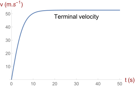
Velocity–time graph for a skydiver reaching terminal velocity. The curve is non-linear, so the area under the graph over a time interval represents displacement and must be estimated when not simple to integrate exactly. This real-world example includes air resistance, which is extra context beyond the syllabus but clarifies why non-linear profiles are common. Source.
Non-linear graph: A graph in which the plotted data do not form a straight line, indicating that the relationship between variables changes with time or magnitude.
In experimental and analytical contexts, such curves frequently occur in real-world motion, such as a car accelerating from rest or a parachutist decelerating under increasing air resistance.
Methods for Estimating Areas Under Curves
There are several effective techniques for estimating areas beneath non-linear graphs. The method chosen depends on the available data, accuracy requirements, and graphical resolution.
1. Counting Squares Method
When using graph paper, the counting squares method provides a straightforward visual approximation.
Divide the area under the curve into grid squares.
Count all fully enclosed squares beneath the curve.
Estimate fractions of partially filled squares.
Multiply the total counted area by the scale factors on each axis to obtain the physical quantity.
This approach, though approximate, is suitable for hand-drawn experimental data or when computational tools are unavailable.
2. Subdivision into Geometric Shapes
The curve can be split into small rectangles, trapezia, or triangles.
Approximate each segment of the curve with a known geometric shape.
Calculate the area of each shape using standard formulae.
Sum the areas to find the total estimated displacement or change in velocity.
EQUATION
—-----------------------------------------------------------------
Trapezium Area (A) = ½ × (a + b) × h
a = One parallel side length (in m/s or m/s²)
b = Other parallel side length (in m/s or m/s²)
h = Width of the strip (in s)
—-----------------------------------------------------------------
This trapezium rule method can produce surprisingly accurate results for smoothly curved data, especially when the number of divisions is large.
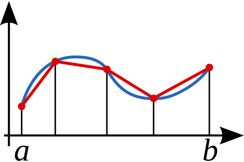
Composite trapezium rule diagram showing how a curved region is partitioned into adjacent trapezia to approximate the total area. Increasing the number of strips usually improves accuracy. The diagram is mathematical but directly supports the graph-area estimation required in this subsubtopic. Source.
3. Numerical Integration Techniques
With digital data, more sophisticated techniques can be applied, such as the trapezoidal rule, Simpson’s rule, or integration functions within spreadsheet software. These methods involve:
Dividing the graph into numerous small intervals.
Calculating the mean value of each section.
Summing the products of mean values and interval widths.
In modern contexts, these calculations are often performed automatically by data-logging software, providing a precise estimate of the area.
Experimental Motion Analysis
To support the estimation of non-linear areas, experimental motion analysis involves capturing motion data using sensors and digital systems. This allows for accurate, continuous measurement of displacement, velocity, and acceleration.
Using Data-Loggers and Sensors
Data-loggers record time-dependent motion data from connected sensors such as light gates, motion sensors, or accelerometers.
Light gates measure time intervals as an object passes through, providing instantaneous velocity.
Ultrasonic motion sensors detect changing distance from the sensor to the object.
Accelerometers directly record acceleration, which can then be integrated to find velocity or displacement.
These sensors produce large data sets with minimal human error, enabling precise plotting of non-linear motion graphs.
ICT in Motion Analysis
The integration of Information and Communication Technology (ICT) has transformed experimental analysis. ICT tools:
Record and display motion graphs in real time.
Allow automatic gradient and area calculations.
Provide options to smooth noisy data and apply curve fitting.
Facilitate immediate visualisation of complex motions, such as oscillations or variable acceleration.
Data-logger: An electronic device that automatically records data over time through sensors, often connected to a computer for analysis.
By combining sensor input and ICT tools, experimental setups can accurately model non-linear motion that would otherwise be too difficult to calculate manually.
Practical Considerations in Estimating Areas
Experimental estimation is not free from uncertainties. The following factors influence accuracy:
Graph resolution: Low-resolution graphs make it difficult to judge gradients and curvature precisely.
Sampling rate: Higher sampling frequency in data-loggers provides more detailed and accurate motion profiles.
Noise and fluctuations: Random variations in sensor readings can distort curves; applying smoothing algorithms or averaging techniques mitigates this.
Measurement timing: Synchronisation errors in starting or stopping timers can cause systematic discrepancies in calculated areas.
EQUATION
—-----------------------------------------------------------------
Displacement (s) = ∫v dt
s = Displacement (m)
v = Velocity (m s⁻¹)
t = Time (s)
—-----------------------------------------------------------------
Although exact integration is rarely performed manually, understanding that area represents this integral reinforces the conceptual link between the graphical method and calculus.
Real-World Applications of Non-Linear Motion Analysis
Estimating areas under non-linear motion graphs is crucial in various experimental and applied contexts:
Vehicle motion tests: Measuring acceleration and braking profiles for safety analysis.
Sports science: Determining an athlete’s performance curve during a sprint or jump.
Physics experiments: Calculating free-fall motion with air resistance or oscillating motion in springs and pendulums.
Engineering systems: Analysing velocity–time data in conveyor systems or rotating machinery.
Each of these applications involves data that rarely fit ideal linear patterns, requiring precise estimation methods supported by technology.
Combining Theory and Experiment
The key educational outcome for students is to relate theoretical understanding of motion with empirical data. Estimating non-linear areas and using ICT tools encourages analytical thinking, quantitative reasoning, and awareness of measurement limitations—core skills in advanced physics study.
Practice Questions
Question 1 (2 marks)
A student records the velocity–time graph of a car accelerating from rest. The graph is curved rather than a straight line.
Explain why the area under this velocity–time graph must be estimated rather than calculated exactly.
Mark scheme:
(1 mark) States that the graph is non-linear or curved, so the relationship between velocity and time is not constant.
(1 mark) Recognises that because of this curvature, the area under the graph cannot be found using a single geometric formula and must be approximated using methods such as counting squares or the trapezium rule.
Question 2 (5 marks)
A motion sensor connected to a data-logger records the velocity of a trolley moving along a track. The velocity–time graph produced is curved.
Describe how the student could estimate the trolley’s displacement using the data recorded. Include reference to the graphical and ICT methods that could be used to improve accuracy.
Mark scheme:
(1 mark) States that displacement is equal to the area under the velocity–time graph.
(1 mark) Describes dividing the curved graph into small strips (trapezia or rectangles) to estimate the total area.
(1 mark) Mentions using the trapezium rule or counting squares as a manual graphical method.
(1 mark) Explains that using a data-logger or computer software allows for automatic calculation of areas or application of numerical integration to increase precision.
(1 mark) Recognises that increasing data sampling rate or using ICT tools reduces random errors and improves the accuracy of the displacement estimate.
FAQ
Increasing the number of recorded data points improves accuracy because each small interval represents a smaller section of the curve, reducing the margin of error in the estimated area.
In practical terms, a higher sampling rate on a data-logger captures more detail of the motion, allowing for finer subdivision when applying numerical methods like the trapezium rule. Too few points can make the graph appear linear over sections that are actually curved, underestimating or overestimating displacement.
However, excessively high sampling rates can introduce noise, so data smoothing or averaging may be necessary for precise results.
The trapezium rule provides a better approximation because it accounts for the changing gradient between two data points. Each trapezium estimates the area under the curve more accurately than a rectangle, which assumes constant velocity within an interval.
While rectangles often overestimate or underestimate the area depending on curve shape, trapezia interpolate between points to create a closer fit.
For strongly curved graphs, using smaller intervals or applying Simpson’s rule can further improve precision, but this requires more complex calculation or ICT tools.
Common sources of uncertainty include:
Graph plotting errors, such as inaccurate scale or reading precision.
Timing inaccuracies, where sensor delays or start/stop errors distort recorded velocity.
Data noise, caused by vibration, background signals, or inconsistent reflections from motion sensors.
Interpolation errors, when assuming linearity between non-linear data points.
To minimise these, students can:
Use high-resolution data-logging equipment.
Apply smoothing techniques or polynomial curve fits.
Repeat trials to identify and reduce random variation.
Modern data-loggers use built-in algorithms that perform numerical integration of velocity–time data. The device sums the small areas under each segment of the curve using rules like the trapezium or Simpson’s rule.
These calculations are performed at high speed using discrete data intervals. The total sum gives displacement, which can be displayed instantly.
This automation removes manual estimation errors and allows users to focus on interpreting results, such as recognising acceleration patterns or identifying anomalies in motion.
Digital analysis using ICT tools offers:
Higher accuracy, as software performs precise numerical integration.
Real-time feedback, allowing immediate adjustments to experiments.
Data storage and manipulation, enabling reanalysis or smoothing of noise.
Automated uncertainty calculations, reducing human error.
Manual methods remain valuable for developing conceptual understanding, but digital systems enhance precision and efficiency, especially when analysing rapidly changing or non-linear motion where hand-drawn approximations are insufficient.
