AP Syllabus focus:
‘Students may use graphing technology to generate slope fields and visualize families of solutions, supporting their understanding of how the differential equation determines solution behavior.’
Technology-generated slope fields provide a dynamic way to observe how a differential equation prescribes local behavior and guides the shapes of entire solution families across the coordinate plane.
Exploring Slope Fields with Graphing Technology
Graphing technology offers a powerful and efficient way to visualize the structure of solutions to a first-order differential equation. When a device or software program constructs a slope field, it places short line segments at selected points whose slopes match the derivative given by the equation. This visualization allows students to see how solutions evolve without explicitly solving the equation.
How Technology Produces Slope Fields
Most graphing utilities operate by evaluating the derivative expression at a grid of points. The software then draws tiny segments whose orientations mirror the local direction of change. Because this process is automated, it enables students to explore many differential equations quickly and observe patterns that may be difficult to see when sketching by hand.
Essential Vocabulary
When working with differential equations in a technological environment, it is important to understand the meaning of solution curve, which is any curve whose tangent at every point matches the slope described by the differential equation.
Solution Curve: A function whose graph aligns with the slope field so that its tangent at each point has slope equal to the value given by the differential equation.
A slope field itself is a collection of these directional indicators, offering a visual summary of all possible solution curves. Technology enhances this summary by generating an accurate and uniform arrangement of segments across the plane.
Setting Up a Differential Equation in Graphing Software
Graphing tools generally require users to input the derivative expression in the form . The program then evaluates this expression over a defined window.

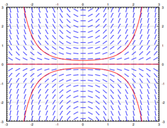
A slope field generated digitally for a differential equation, where each segment's orientation corresponds to the slope value given by , allowing students to observe underlying solution behavior. Source.
= Rate of change of with respect to
= Derivative formula defining slope values
After the equation is entered, the user can adjust parameters such as window size, grid density, or the spacing of the displayed slope segments. This flexibility allows students to focus on particular features, such as regions where slope behavior changes rapidly or where solutions appear to converge.
A natural pause occurs here before considering how students interact with the generated field.
Visualizing Families of Solutions
Once the slope field appears, graphing technology often allows students to superimpose solution curves by selecting a point on the screen.

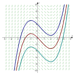
A slope field with multiple solution curves overlaid, each curve's tangent matching the local slope segments and demonstrating how digital tools reveal entire families of solutions. Source.
The software traces the corresponding solution curve numerically, following the pattern of slope segments. This capability reveals that differential equations do not produce a single solution but rather a family of solutions.
Family of Solutions: A collection of solution curves, often differing by a constant, that all satisfy the same differential equation.
By visually displaying multiple members of this family, technology helps clarify the idea that a differential equation describes a system of infinitely many possible solution paths.
Linking Slope Fields to Differential Equation Behavior
Digital visualization highlights important qualitative features of a differential equation. Students can use the generated field to observe how solutions behave in different regions of the plane. Key aspects include:
Direction patterns that reveal whether slopes increase, decrease, or remain constant across the plane.
Visual evidence of equilibrium tendencies, where slopes appear horizontal or nearly horizontal.
Regions of rapid change, where slope magnitudes grow large, indicating steep solution segments.
Areas where solutions diverge or converge, showing how sensitive the differential equation is to initial conditions.
These observations deepen conceptual understanding because they directly link symbolic expressions to geometric and qualitative representations.
Using Technology to Support Conceptual Reasoning
Technology-generated slope fields serve as a bridge between symbolic work and visual intuition. Students can:
Investigate how modifying a parameter in a differential equation alters the entire field of slopes.
Compare slope fields for different equations to see how structural differences influence solution behavior.
Observe the continuity and smoothness in solution paths that arise naturally from the local slope information.
Identify how long-term trends emerge from repeated local behavior encoded in the derivative expression.
This type of reasoning is uniquely supported by technology, which produces precise representations faster and more accurately than manual sketches. Having immediate access to a full slope field also encourages experimentation—an important part of learning differential equations.
Practical Benefits of Using Graphing Technology
Relying on technology to explore slope fields provides several instructional advantages:
It reduces time spent on tedious drawing, allowing students to focus on interpretation.
It produces consistent scales and segment lengths, preventing hand-drawn inaccuracies from obscuring patterns.
It highlights relationships between initial conditions and their resulting solution curves.
It assists in connecting symbolic forms of differential equations to real-world behavior, strengthening conceptual understanding.
Because the AP syllabus explicitly supports the use of technology for slope field visualization, students are encouraged to integrate these techniques into their study of differential equations. By interpreting these graphical outputs, they gain valuable experience in understanding how the derivative structure of an equation shapes the behavior of its solutions.
FAQ
Altering the viewing window changes which region of the differential equation’s behaviour is visible. A wider window shows more global structure, while a narrower window highlights local slope variations.
Adjusting the vertical or horizontal scale can make slopes appear steeper or flatter, influencing how easily patterns such as symmetry or equilibrium tendencies can be spotted.
A well-chosen window helps prevent distortion and allows solution behaviour to be interpreted more reliably.
Grid density determines how many points the software samples when drawing slope segments.
Higher density adds detail but can clutter the display.
Lower density reduces visual noise but may obscure regions where slope behaviour changes rapidly.
A balanced density helps students recognise meaningful patterns without overwhelming the graph.
Different tools may use varying numerical sampling methods, rounding behaviours, or segment lengths.
Some programs automatically adjust scaling or normalise steep slopes, while others preserve raw derivative values.
These differences rarely affect qualitative interpretation but can change the clarity or uniformity of the slope field.
By tapping or selecting multiple nearby points, students can generate several solution curves on the same slope field.
If initially close curves diverge quickly, the equation shows high sensitivity to initial conditions.
If curves stay close over a long interval, sensitivity is low.
This visual comparison helps highlight structural features that are not obvious from the derivative expression alone.
Students can plot slope fields for different equations side by side or toggle between them.
Key differences to observe include:
• How slope signs change across the plane
• Whether solutions appear to converge, diverge, or level off
• How symmetry or asymmetry arises from the derivative expression
This comparison deepens understanding of how structural changes in an equation alter solution behaviour.
Practice Questions
Question 1 (1–3 marks)
A graphing tool displays the slope field for the differential equation dy/dx = x – y. A student clicks the point (1, 2), and the software draws a solution curve through that point.
(a) Explain what the slope field represents at the point (1, 2).
(b) State how the technology determines the shape of the solution curve passing through (1, 2).
Question 1
(a) 1 mark for stating that the small line segment shows the slope given by substituting x = 1 and y = 2 into the differential equation.
(b) 1–2 marks for explaining that the software follows the local slopes in the field or uses numerical methods to trace a curve whose tangent at each point matches the slope indicated by the differential equation.
Question 2 (4–6 marks)
A student uses graphing technology to display the slope field for a first-order differential equation. The field shows that slopes are positive for x > 0 and negative for x < 0, and that slopes become steeper as the distance from the x-axis increases.
(a) Describe how graphing technology uses the differential equation to produce this slope field.
(b) Explain what the observed slope pattern suggests about the long-term behaviour of solution curves starting above and below the x-axis.
(c) Comment on how the use of technology helps students understand families of solutions for the differential equation.
Question 2
(a) 1–2 marks for stating that the software evaluates the derivative at points in a grid and draws short line segments with the corresponding slope.
(b) 2–3 marks for explaining that positive slopes to the right and negative slopes to the left imply curves rise for x > 0 and fall for x < 0, while increasing steepness away from the x-axis suggests solutions diverge from the axis as x increases in magnitude.
(c) 1 mark for noting that technology shows multiple possible solution paths and helps visualise how initial conditions lead to different curves within the same family.

