1.3.2 Opportunity Cost and Trade-Offs on the PPC

AP Syllabus focus: ‘The PPC illustrates scarcity, trade-offs, and opportunity cost, and it can be used to calculate opportunity cost from graphs or tables.’

A production possibilities curve (PPC) turns the abstract idea of scarcity into a visual model. Its key purpose is to show trade-offs and to measure opportunity cost when resources shift between two outputs.

Core Ideas on the PPC

Scarcity and trade-offs on the curve

A PPC shows the maximum attainable combinations of two goods (or categories of goods) that can be produced with limited resources and a given technology.

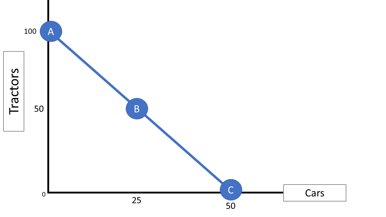
A linear production possibilities curve (PPC) showing the maximum feasible combinations of two goods (cars on the horizontal axis and tractors on the vertical axis). Points A, B, and C lie on the frontier, illustrating productively efficient bundles achievable with the economy’s current resources and technology. Source

Because resources are scarce, producing more of one good requires producing less of the other, creating a trade-off.

Opportunity cost: The value of the next best alternative given up when making a choice.

On a PPC, the trade-off is represented by movement along the curve: reallocating resources toward one output forces a reduction in the other output.

What “opportunity cost” means on a PPC

Opportunity cost on the PPC is measured in units of the other good forgone. If the economy moves from one point on the PPC to another point on the PPC and gains additional units of Good X, it must give up some units of Good Y. That forgone amount of Y is the opportunity cost of the increase in X over that range.

This is why the PPC is especially useful: it connects a choice (“more X”) to a concrete cost (“less Y”).

Calculating Opportunity Cost from a Graph

The slope-as-cost idea

On a PPC graph (with Good X on the horizontal axis and Good Y on the vertical axis), the slope between two points captures the trade-off. Interpreting the slope carefully is essential:

The slope is typically negative (more X means less Y).
The absolute value of the slope tells you how much Y is given up per additional unit of X over a specified movement.

A common AP Micro interpretation is “units of Y per unit of X,” which is the opportunity cost of producing X (over that segment).

$Opportunity\ Cost\ of\ X = \dfrac{\Delta Y}{\Delta X}$

$\Delta Y$ = Change in Good Y (units forgone when moving toward more X)

$\Delta X$ = Change in Good X (additional units produced)

Because the PPC trade-off can differ across ranges, always compute using the two points relevant to the movement being described, not by assuming one constant cost everywhere.

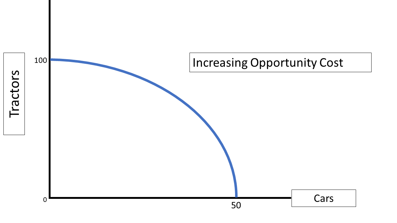
A bowed-out (concave) PPC illustrating increasing opportunity cost: as production shifts toward more of the good on the horizontal axis, the curve becomes steeper. The changing slope implies that the opportunity cost (units of the other good forgone per extra unit gained) rises as resources are reallocated to less-suited uses. Source

Reading the graph correctly (process)

Identify the two points (starting bundle and ending bundle).
Compute the change in each good: $\Delta X$ and $\Delta Y$ .
Interpret opportunity cost as the forgone output of the other good:
- For more X: opportunity cost is units of Y given up.
- For more Y: opportunity cost is units of X given up.
State the cost with clear units (for example, “Y per additional unit of X”).

Calculating Opportunity Cost from a Table

What PPC tables represent

A PPC table lists feasible production combinations (bundles) of two goods.

Each row is a point on the PPC (or sometimes includes interior points if the table also shows inefficiency). When the table gives PPC points, opportunity cost is found by comparing two adjacent bundles or two specified bundles.

Interpreting “per unit” opportunity cost from a table (process)

Choose the two bundles being compared (often consecutive rows).
Determine how many units of one good increase.
Determine how many units of the other good decrease.
Express opportunity cost as a ratio:
- “Giving up ___ units of Y to gain ___ units of X,” and, if requested, convert to “per 1 unit of X.”

In AP Micro, this ratio-based reasoning is the same logic as using slope on a graph; the table is simply a different representation of the same trade-off.

Key Pitfalls to Avoid

Mixing up direction: the opportunity cost of more X is what you give up of Y, not what you gain of X.
Forgetting units: opportunity cost should be stated in units of the alternative good.
Assuming constant opportunity cost without being told: compute it over the specific movement described by the graph segment or table interval.

FAQ

Two goods keep the trade-off visible on a 2D graph.

With more goods, the same idea extends to higher dimensions, but it becomes harder to visualise.

No. On a PPC, opportunity cost is measured in foregone output of the other good.

Money prices may reflect opportunity costs, but the PPC itself is a real-output model.

It means the opportunity cost of a small (next) increase in one good.

Graphically, it corresponds to the slope at a point (rather than between two distant points).

Reading values off axes can introduce approximation error.

Using clearly labelled points (or exact table values) reduces rounding issues and improves precision.

Yes, but interpretation must keep units explicit.

Opportunity cost becomes “services forgone per extra ton,” so careful unit labelling is essential when comparing statements.

Practice Questions

Question 1 (1–3 marks) A PPC shows combinations of Good X and Good Y. Explain what opportunity cost means when moving along the PPC from a point with more Y to a point with more X. (2 marks)

Defines opportunity cost as the next best alternative forgone (1).
Applies to PPC movement: producing more X requires sacrificing some Y, so forgone Y is the opportunity cost of extra X (1).

Question 2 (4–6 marks) A PPC table lists two attainable bundles: Bundle A produces $(X_A, Y_A)$ and Bundle B produces $(X_B, Y_B)$ , where $X_B>X_A$ and $Y_B<Y_A$ . Describe how to calculate the opportunity cost of increasing X from A to B and how this relates to the PPC’s slope. (5 marks)

Identifies changes: $\Delta X = X_B-X_A$ and $\Delta Y = Y_B-Y_A$ (1).
States that the amount of Y forgone is $-(\Delta Y)$ when $\Delta Y<0$ (1).
Computes opportunity cost of the increase in X as $\dfrac{\text{Y forgone}}{\Delta X} = \dfrac{-\Delta Y}{\Delta X}$ (1).
Links to graph: this ratio corresponds to the (absolute value of the) slope between the two PPC points (1).
Interprets meaning with correct units, e.g., “units of Y per additional unit of X” (1).

Try All Topic Practice Questions

Written by:

Dave

Profile

Cambridge University - BA Hons Economics

Dave is a Cambridge Economics graduate with over 8 years of tutoring expertise in Economics & Business Studies. He crafts resources for A-Level, IB, & GCSE and excels at enhancing students' understanding & confidence in these subjects.