These notes explain how to extract opportunity cost, absolute advantage, and comparative advantage directly from common data formats on the AP exam—simple production tables and production possibilities curves (PPCs).

Core concepts you must identify from data

Opportunity cost is the foundation: comparative advantage is determined by comparing opportunity costs, not by comparing total output.

Absolute advantage comes from higher productivity (more output per fixed input), but it does not decide who should specialise.

Comparative advantage is always a relative concept: you must compute and compare opportunity costs across producers.

Finding advantage from production tables (maximum outputs)

A typical table gives each producer’s maximum output of two goods (often assuming the same time, labour, or resources). Use it to compute opportunity costs and advantages.

Process: from table to opportunity cost

• Confirm the table shows maximum amounts of each good using the same resource base (e.g., “per day,” “per worker,” “per hour”).

• Compute each producer’s opportunity cost of one unit of a good in terms of the other good.

• Compare opportunity costs to determine comparative advantage.

• Compare maximum outputs to determine absolute advantage.

When a table only lists two endpoints (all-X or all-Y), treat it like a straight-line trade-off between those endpoints for opportunity-cost purposes: compare “what you give up” to “what you gain.”

How to identify each advantage from the table

• Absolute advantage (in X): the producer with the larger maximum X.

• Absolute advantage (in Y): the producer with the larger maximum Y.

• Comparative advantage (in X): the producer with the lower $OC$(1 unit of X).

• Comparative advantage (in Y): the producer with the lower $OC$(1 unit of Y) (equivalently, the other producer if there are only two goods).

Finding advantage from PPCs

A PPC displays feasible combinations of two goods from a fixed set of resources and technology.

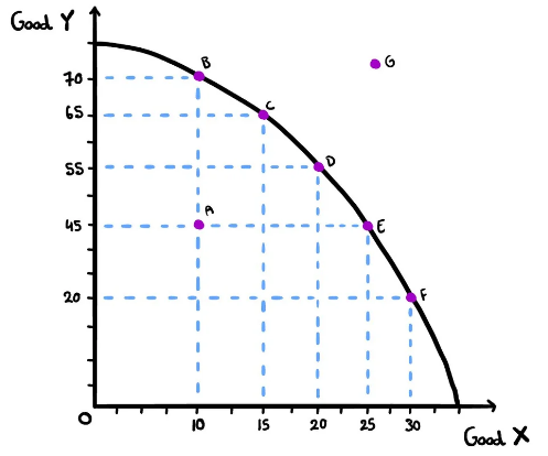
This PPC diagram clearly distinguishes feasible points on the curve from inefficient points inside the curve and unattainable points outside it. Because the PPC is the boundary of maximum feasible combinations, it visually reinforces that opportunity cost arises when moving along the frontier, not by jumping to impossible points. The labeled points make it straightforward to practice “read the graph first, then compute the trade-off” under exam conditions. Source

You can read opportunity costs from endpoints and slopes.

Step 1: read intercepts (maximum outputs)

• The x-intercept is the maximum amount of the x-axis good if all resources go to it.

• The y-intercept is the maximum amount of the y-axis good if all resources go to it.

Use these intercepts to identify absolute advantage the same way you would from a table: higher intercept for a good implies higher maximum output for that good.

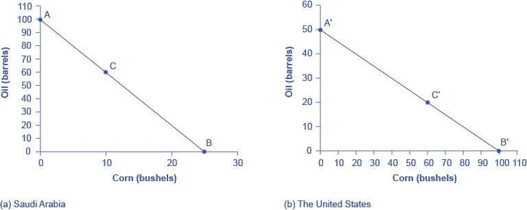
This OpenStax figure pairs maximum-output information with production possibilities frontier (PPF) graphs, making it easy to see intercepts as “all of one good” endpoints. The diagram visually connects opportunity cost to the PPF’s slope: gaining more of one good requires giving up some of the other. This is the graphical basis for computing opportunity costs and then identifying comparative advantage by comparing those trade-offs across producers. Source

Step 2: compute opportunity cost from the PPC

On a PPC, opportunity cost is the trade-off between goods:

• Moving right (more x-axis good) typically means moving down (less y-axis good).

• The opportunity cost of gaining X is measured by the drop in Y needed to obtain that gain in X.

For a straight-line PPC, opportunity cost is constant and equals the (absolute value of the) slope. For a curved PPC, opportunity cost is found by the slope over the specific range you are moving through.

Step 3: determine comparative advantage from slopes

To identify comparative advantage using PPCs:

• Compute (or compare) each producer’s opportunity cost of producing one good.

• The producer with the lower opportunity cost in a good has the comparative advantage in that good.

Practical graph-reading cues:

• If Producer A’s PPC is relatively flatter than Producer B’s, A gives up less Y per extra X, so A tends to have comparative advantage in the x-axis good (over that range).

• If Producer A’s PPC is relatively steeper, A gives up more Y per extra X, so A tends to have comparative advantage in the y-axis good (over that range).

Common pitfalls when using tables and PPCs

• Don’t confuse absolute with comparative advantage: “can produce more” is not the same as “has lower opportunity cost.”

• Keep units consistent (per hour vs per day). Inconsistent bases invalidate comparisons.

• For curved PPCs, don’t assume one opportunity cost applies everywhere; use the relevant segment or stated movement.

• Comparative advantage must be determined from ratios/trade-offs, not from differences in outputs.