The supply-and-demand model is the core tool for explaining how competitive markets determine prices and quantities. It helps you compare markets, predict changes over time, and organise real-world shocks into clear economic logic.

What the Supply-and-Demand Model Does

The supply-and-demand model predicts the market price and quantity of a good using two relationships:

• Demand: buyers’ willingness and ability to purchase at different prices

• Supply: sellers’ willingness and ability to produce and sell at different prices

It is a comparative statics framework: you compare an initial outcome to a new outcome after some change (a “shock”) to market conditions, holding other factors constant (ceteris paribus).

In AP Microeconomics, this model is typically used for perfectly competitive markets, where many buyers and sellers interact and no single participant controls price.

Building the Model: Demand and Supply

Demand: what shapes buyers’ behavior

A demand curve shows the relationship between price and quantity demanded, holding other determinants constant. When those other determinants change, demand shifts.

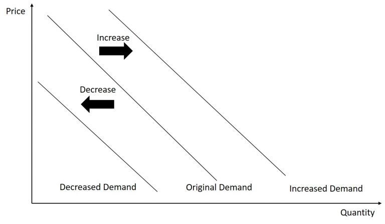
A demand-shift diagram showing three demand curves: decreased demand (left), original demand (middle), and increased demand (right). It emphasizes that a change in a demand determinant moves the entire demand relationship (a shift), rather than causing a movement along a single curve due to the good’s own price changing. Source

Common determinants of demand (causes of shifts) include:

• Income (especially important for normal vs inferior goods)

• Tastes and preferences

• Prices of related goods (substitutes and complements)

• Expectations about future prices or income

• Number of buyers in the market

Using the model means separating:

• A movement along the demand curve (caused by a change in the good’s own price)

• A shift of the demand curve (caused by a change in a determinant other than the good’s own price)

Supply: what shapes sellers’ behavior

A supply curve shows the relationship between price and quantity supplied, holding other determinants constant. When those other determinants change, supply shifts.

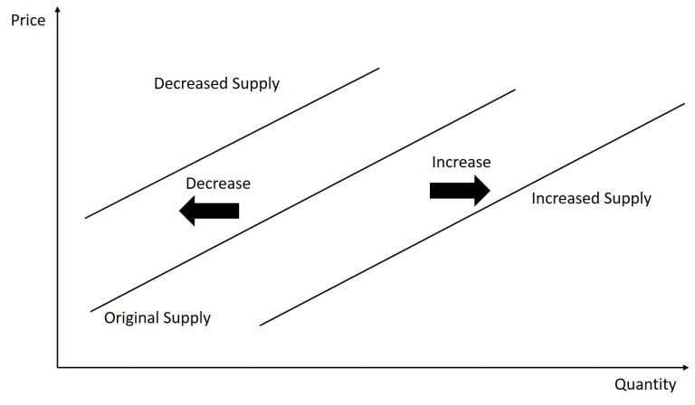
A supply-shift diagram showing decreased supply (left), original supply (middle), and increased supply (right) on Price–Quantity axes. This helps visualize how changes in production conditions (costs, technology, policy, number of sellers) shift the entire supply curve, changing the quantity supplied at every price. Source

Common determinants of supply include:

• Input prices (costs of labour, raw materials, energy)

• Technology and productivity

• Taxes/subsidies and regulation that affect costs (treated as cost shifts)

• Expectations about future prices or input costs

• Number of sellers in the market

As with demand:

• A movement along supply comes from a change in the good’s own price

• A shift of supply comes from changes in costs or production conditions

Reading the Graph: Price, Quantity, and the Market Outcome

On the standard graph:

• Vertical axis: Price (P)

• Horizontal axis: Quantity (Q)

• The intersection of supply and demand indicates the model’s predicted market outcome: the equilibrium price and quantity.

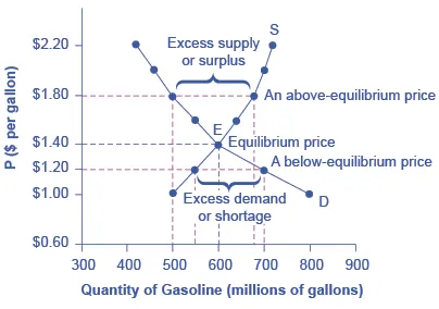
A standard supply-and-demand equilibrium graph: the demand curve (D) and supply curve (S) intersect at point $E$, determining the equilibrium price and quantity. The diagram also shows that prices above equilibrium generate a surplus (excess supply), while prices below equilibrium generate a shortage (excess demand), illustrating how market pressures push price back toward equilibrium. Source

Even when you are not doing calculations, it is useful to express equilibrium as the condition that the quantity buyers want equals the quantity sellers want at that price.

The key skill is translating a real-world change into “demand shifts right/left” or “supply shifts right/left,” then using the new intersection to infer how P and Q change.

Using the Model to Explain Differences Across Markets

The model explains why two markets can have very different prices and quantities for similar goods. Differences come from underlying demand and supply conditions, such as:

• Demand differences: higher incomes, stronger preferences, larger populations, or fewer substitutes can push demand higher, raising the predicted price and quantity (depending on supply).

• Supply differences: cheaper inputs, better technology, favourable climate/locations, or more sellers can push supply higher, lowering the predicted price and raising the predicted quantity (depending on demand).

Importantly, you cannot conclude “high price means high demand” without also considering supply. A high price could reflect strong demand, weak supply, or both.

Using the Model to Explain Changes Over Time (Comparative Statics)

To use the model cleanly, follow a consistent process:

• Identify the market (be precise about the good and geographic/time boundaries).

• Identify the shock (what changed in the world?).

• Decide whether the shock changes demand or supply (or both).

• Determine the direction of the shift:

  • Demand right = higher demand at every price; demand left = lower demand at every price

  • Supply right = greater supply at every price; supply left = lower supply at every price

• Compare the old and new intersections to infer changes in:

  • Equilibrium price

  • Equilibrium quantity

When both curves shift at once, the model still works: it usually gives a clear direction for one variable (price or quantity) and an ambiguous direction for the other unless you know which shift is larger. This is one reason the supply-and-demand model is powerful for explaining real markets: multiple forces often operate simultaneously.