Two-dimensional kinematics becomes manageable when you treat motion along perpendicular axes separately. This approach relies on careful component bookkeeping, consistent sign conventions, and recognising that the same time interval applies to both axes.

Key Idea: Components Make 2D Motion “Two 1D Problems”

In two dimensions, position, velocity, and acceleration each have an x-part and a y-part. You analyse each axis with familiar one-dimensional kinematics, then combine results to describe the full motion.

A central benefit is that motion in the x-direction does not mathematically “mix” with motion in the y-direction in the kinematic equations; they share only the same time variable.

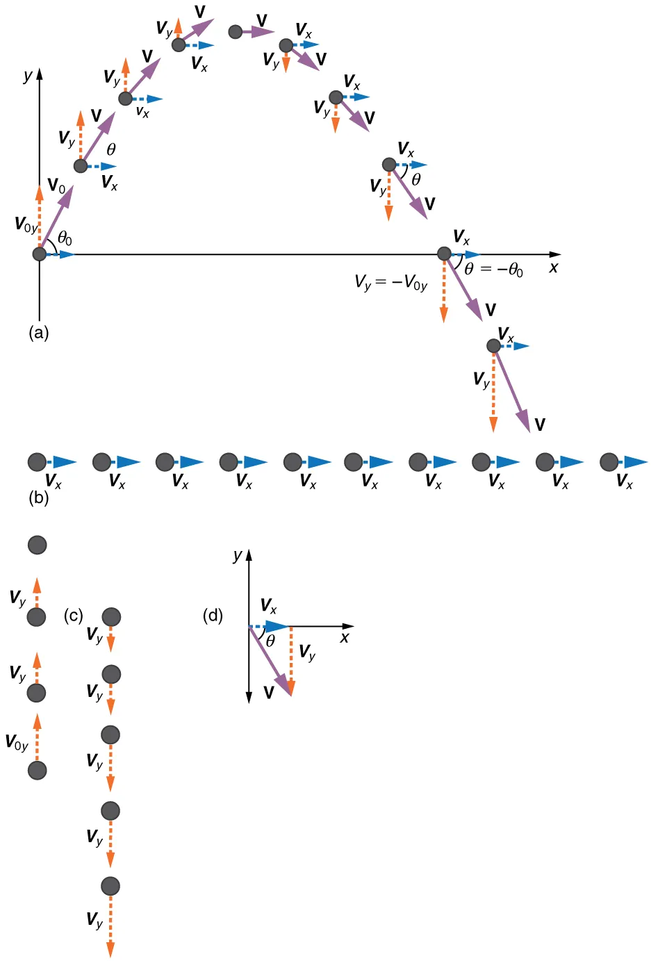
A multi-panel projectile-motion diagram showing the full trajectory with the velocity vector decomposed into $v_x$ and $v_y$, plus separate panels emphasizing that $v_x$ stays constant (when $a_x=0$) while $v_y$ changes under constant downward acceleration. This is a visual proof of “two 1D problems, same time,” which is exactly what you leverage when solving AP Physics 1 component kinematics. Source

How to Break Motion Into Components (Workflow)

1) Choose axes and define signs

• Pick perpendicular axes (commonly x horizontal, y vertical).

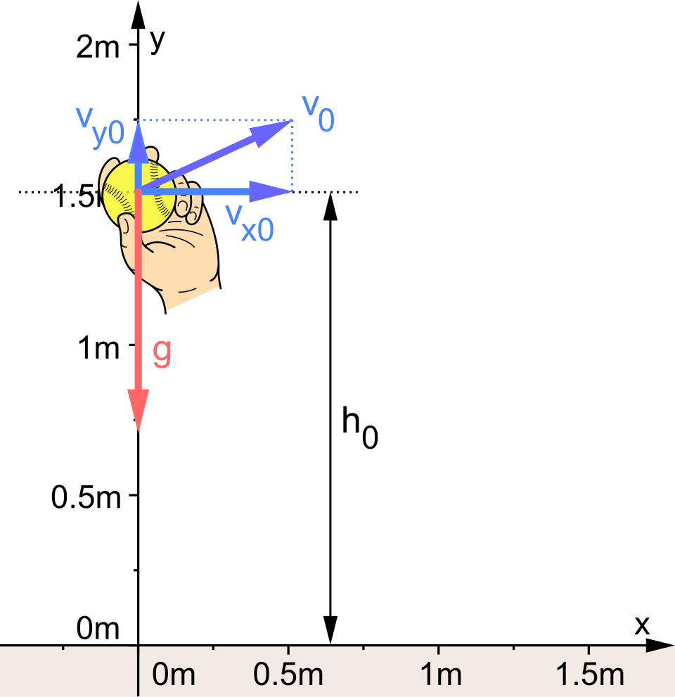
A projectile-motion coordinate setup showing the $x$- and $y$-axes, the projectile’s position relative to the origin, and the direction of gravitational acceleration. This kind of diagram is the standard “first sketch” that makes later component equations unambiguous. Source

• Define positive directions and stick to them.

• Record initial conditions separately: initial position, initial velocity, and acceleration in x and y.

2) Write what you know for each axis

Treat each axis independently:

• Along x: track displacement in x, velocity in x, acceleration in x.

• Along y: track displacement in y, velocity in y, acceleration in y.

The key constraint linking the axes is that the elapsed time is the same for both x and y descriptions.

3) Apply one-dimensional kinematics along each axis

Use any one-dimensional constant-acceleration relationships (when acceleration is constant) separately for x and y. For algebra-based problem solving, the most important habit is matching the right variables to the right axis and never combining x-quantities into y-equations.

4) Recombine only at the end (if needed)

Sometimes you need the overall (resultant) velocity or displacement.

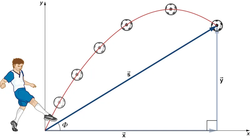
A displacement-vector diagram where the total displacement is the hypotenuse of a right triangle whose legs are the horizontal and vertical components. It illustrates how magnitudes and directions are recovered from perpendicular components using geometry after the component-wise kinematics are finished. Source

In that case, combine the perpendicular components using geometry:

• The resultant magnitude depends on both components.

• The direction depends on the ratio of the components and the sign conventions you chose.

Interpreting What “Independent Axes” Really Means

“Independent” does not mean “unrelated in the real world”; it means the mathematical update rules are separate:

• A change in x-velocity comes from x-acceleration only.

• A change in y-velocity comes from y-acceleration only.

• The time interval is shared, so timing conditions (like “when it reaches a certain height” or “after 3 seconds”) affect both axes simultaneously.

Common Pitfalls to Avoid

• Mixing component labels (using a y-displacement in an x-equation).

• Flipping signs mid-problem (changing what “positive y” means).

• Combining components too early (finding a resultant speed before solving for the needed time).

• Forgetting that initial conditions apply per axis (vx0 and vy0 can be very different).