Exponential Motion with Linear Drag (2.9.4) | AP Physics C: Mechanics Notes

AP Syllabus focus: 'For a resistive force proportional to velocity, position, velocity, and acceleration are exponential functions with asymptotes set by the initial conditions and the forces involved.'

Linear drag causes motion to change quickly at first and then level off. In AP Physics C Mechanics, the key idea is that a force proportional to velocity produces exponential time dependence.

Linear drag as a model

A linear drag force is a resistive force whose magnitude is proportional to the object's speed and whose direction is opposite the velocity. This model is most useful when the motion is one-dimensional and the drag is weak enough that proportionality to $v$ is a good approximation.

Linear drag: A resistive force modeled as directly proportional to velocity and opposite in direction to the motion.

In a chosen positive direction, the drag force is written with a minus sign because it opposes the motion along that axis.

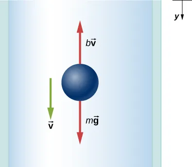
Free-body diagram for 1D motion with linear drag: the velocity vector points downward while the drag force $b\vec{v}$ points upward, opposing the motion. This picture reinforces why the drag term enters as $-bv$ along the chosen axis and why the net force (and thus acceleration) decreases as the speed increases toward terminal speed. Source

$F_d=-bv$

$F_d$ = drag force along the chosen axis, in $N$

$b$ = positive drag constant, in $kg/s$

$v$ = velocity, in $m/s$

When linear drag acts together with a constant force $F_0$ in the positive direction, Newton's second law gives a first-order differential equation. Its solution is exponential because the rate at which velocity changes depends on how far the current velocity is from its long-time value.

Velocity approaches an asymptote

The most useful way to write the velocity is in terms of an asymptotic velocity and a time constant. The asymptotic velocity is the value approached at large times, and the time constant sets how quickly the approach happens.

$v(t)=v_\infty+(v_0-v_\infty)e^{-t/\tau}$

$v(t)$ = velocity at time $t$ , in $m/s$

$v_\infty$ = asymptotic velocity, in $m/s$

$v_0$ = initial velocity at $t=0$ , in $m/s$

$t$ = time, in $s$

$\tau$ = time constant, in $s$

$v_\infty=\dfrac{F_0}{b}$

$F_0$ = constant external force, in $N$

$b$ = drag constant, in $kg/s$

$\tau=\dfrac{m}{b}$

$m$ = mass, in $kg$

This form makes the physics easy to interpret. If $v_0>v_\infty$ , the exponential term is positive and the velocity decays downward toward the asymptote. If $v_0<v_\infty$ , the exponential term is negative and the velocity rises upward toward it. In either case, the difference $v-v_\infty$ shrinks by the factor $e^{-t/\tau}$ . After one time constant, the remaining difference is $1/e$ of its initial value.

Acceleration and position have the same exponential signature

Because acceleration is the time derivative of velocity, it carries the same exponential factor.

Position comes from integrating velocity, so it also contains the same exponential term, although a constant-force case also includes a linear term in time.

$a(t)=-\dfrac{v_0-v_\infty}{\tau}e^{-t/\tau}$

$a(t)$ = acceleration at time $t$ , in $m/s^2$

$x(t)=x_0+v_\infty t+\tau(v_0-v_\infty)(1-e^{-t/\tau})$

$x(t)$ = position at time $t$ , in $m$

$x_0$ = initial position at $t=0$ , in $m$

$v_\infty$ = asymptotic velocity, in $m/s$

$\tau$ = time constant, in $s$

The acceleration always tends to zero as $t$ becomes large. That is a central feature of linear-drag motion: as the object approaches its asymptotic velocity, the net force and therefore the acceleration fade away exponentially.

The position function needs careful interpretation. If a constant force is present, $x(t)$ does not usually approach a fixed number. Instead, it approaches a straight-line behavior with slope $v_\infty$ . The exponential term only describes how the motion settles into that long-time behavior. If there is no constant force, then $v_\infty=0$ , so the position can approach a finite limiting value.

How initial conditions and forces set the asymptotes

The shape of the motion is controlled by two inputs: the initial conditions and the forces involved. The initial conditions, such as $x_0$ and $v_0$ , determine where the graphs start and whether the exponential term begins positive or negative. The forces determine the asymptotes through $F_0$ and $b$ .

Asymptote: A value or line that a function approaches as time increases.

A larger drag constant $b$ produces a smaller time constant $m/b$ , so the motion settles more quickly. A larger mass makes the time constant larger, so the exponential change is more gradual. A larger constant force increases $v_\infty=F_0/b$ , shifting the long-time velocity upward in the positive direction.

Graphically, the velocity-time curve approaches a horizontal asymptote at $v_\infty$ . The acceleration-time curve approaches zero with the same decay constant. The position-time curve contains the same exponential signature, but its asymptote depends on the force situation: it can approach a fixed position when the long-time velocity is zero, or a straight line when the long-time velocity is nonzero.

For AP Physics C, the important recognition skill is not just writing formulas. You should be able to look at a function containing $e^{-t/\tau}$ and identify what it means physically: the motion changes rapidly at first, the rate of change slows over time, and the object approaches a long-time behavior determined by the drag, the applied force, and the initial state.

FAQ

It is usually a good approximation at relatively low speeds, especially in situations where the resistive force is dominated by viscous effects rather than turbulent flow.

For many real objects moving quickly through air, drag is better modelled as proportional to $v^2$, so the linear model is mainly an idealisation or a low-speed approximation.

If the mass $m$ is known, you can determine the time constant $\tau$ from the way the velocity approaches its asymptotic value, then use $b=\dfrac{m}{\tau}$.

If a constant force is also known, you could instead measure the asymptotic velocity and use $b=\dfrac{F_0}{v_\infty}$. In practice, using both methods can help check consistency.

Yes. If the initial velocity is opposite to the direction of the long-time motion, the object may slow to zero and then reverse direction.

The drag force changes sign automatically because it is proportional to $-v$. That means it always opposes the instantaneous motion, even after the reversal.

A useful trick is to look at the difference from the asymptote, such as $v-v_\infty$. For linear drag, that difference should decay like a single exponential.

If you plot $\ln |v-v_\infty|$ against $t$, the result should be a straight line with slope $-\dfrac{1}{\tau}$, provided the model is appropriate and the data are clean enough.

It can, if the resistive force is modelled in vector form as $\vec{F}_d=-b\vec{v}$ and the other forces are constant. Then each velocity component can show the same exponential approach pattern.

However, if the drag depends on speed in a more complicated way, or if the force direction changes with time, the component equations may no longer reduce to simple single-exponential forms.

Practice Questions

An object moving along the $x$ -axis under a constant force and linear drag has velocity $v(t)=v_\infty+(v_0-v_\infty)e^{-t/\tau}$ . State the value approached by $v(t)$ as $t\to\infty$ and the value approached by $a(t)$ as $t\to\infty$ .

1 mark: States that $v(t)\to v_\infty$
1 mark: States that $a(t)\to 0$

A particle of mass $m$ moves along the $x$ -axis under a constant force $F_0$ and a resistive force $-bv$ . At $t=0$ , its position and velocity are $x_0$ and $v_0$ . The velocity is $v(t)=v_\infty+(v_0-v_\infty)e^{-t/\tau}$ , where $v_\infty=\dfrac{F_0}{b}$ and $\tau=\dfrac{m}{b}$ .

(a) Obtain an expression for the acceleration $a(t)$ .

(b) Obtain an expression for the position $x(t)$ .

(a)

1 mark: Correct differentiation of $v(t)$
1 mark: $a(t)=-\dfrac{v_0-v_\infty}{\tau}e^{-t/\tau}$ or equivalent

(b)

1 mark: Correct integration of $v(t)$ with constant of integration
1 mark: $x(t)=x_0+v_\infty t+\tau(v_0-v_\infty)(1-e^{-t/\tau})$

(c)

1 mark: States that $x(t)$ approaches a straight line with slope $v_\infty$ for large $t$ , or equivalent wording

Try All Topic Practice Questions

Written by:

Dr Shubhi Khandelwal

Qualified Dentist and Expert Science Educator

Shubhi is a seasoned educational specialist with a sharp focus on IB, A-level, GCSE, AP, and MCAT sciences. With 6+ years of expertise, she excels in advanced curriculum guidance and creating precise educational resources, ensuring expert instruction and deep student comprehension of complex science concepts.

Qualified Dentist and Expert Science Educator

AP Physics C: study notes

2.9.4 Exponential Motion with Linear Drag

Linear drag as a model

Velocity approaches an asymptote

Acceleration and position have the same exponential signature

How initial conditions and forces set the asymptotes

FAQ

Practice Questions

Hire a tutor