The normal distribution is central in AP Statistics because it models numerous real-world phenomena and provides a foundation for interpreting standardized scores and probability-based conclusions.

The Nature of the Normal Distribution

The normal distribution is a theoretical model describing how some quantitative variables are distributed. It is characterized by its smooth, continuous curve and its distinctive mound-like appearance. This distribution is most useful for variables influenced by many small, independent factors—such as height, measurement errors, or physiological traits. Because of its widespread applicability, recognizing its structural features is essential for statistical reasoning.

A distribution in statistics describes the frequency of values for a variable. When that distribution follows a particular pattern—specifically, a bell shape—it is considered normal. The bell shape signals that most observations cluster around a central value, with fewer observations appearing as values move toward the extremes.

Shape: Mound-Shaped and Symmetric

One hallmark of the normal distribution is its symmetry. Symmetry means that the left and right sides of the distribution mirror one another around the center point. This symmetry implies that low values and high values occur with balanced frequency, and that the central region contains the greatest density of observations.

When discussing shape in AP Statistics, students focus on the concept of a mound-shaped curve, where frequencies rise to a single peak in the center and taper evenly on both sides. In a perfectly normal distribution, this symmetry is exact, making it easier to interpret standardized scores and make probabilistic statements.

Parameters of a Normal Distribution

A normal distribution is defined by two numerical characteristics, or parameters: the mean and the standard deviation.

The parameter μ (mu) represents the mean, or center, of the distribution, while σ (sigma) represents the standard deviation, a measure of spread.

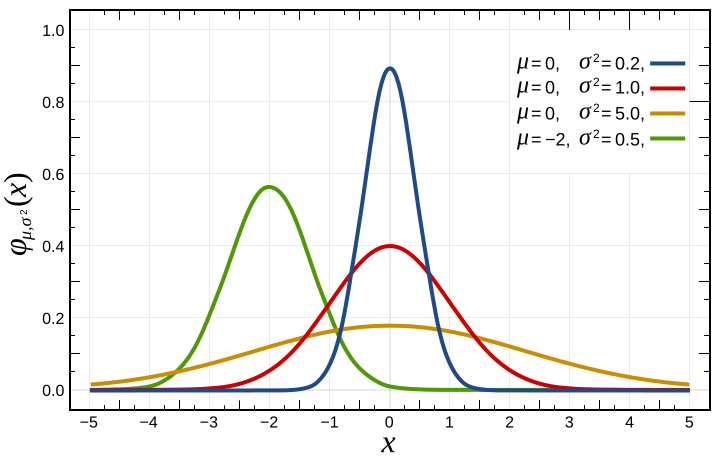
A set of normal curves with different means and standard deviations, showing how μ shifts the curve horizontally and σ stretches or compresses its spread. Source.

EQUATION

Because a normal distribution is fully described by μ and σ, understanding these parameters helps students interpret patterns, compare distributions, and assess deviations from typical values.

A normal sentence follows here to maintain required spacing before another formal block.

Empirical Rule: Understanding Spread in a Normal Model

A defining feature of normally distributed data is its predictable spread. The empirical rule (or 68–95–99.7 rule) describes how data fall relative to the mean when the distribution is approximately normal. This rule is essential for estimating probabilities and making informal judgments about extremity.

This approximate pattern is summarized by the empirical rule (68–95–99.7 rule).

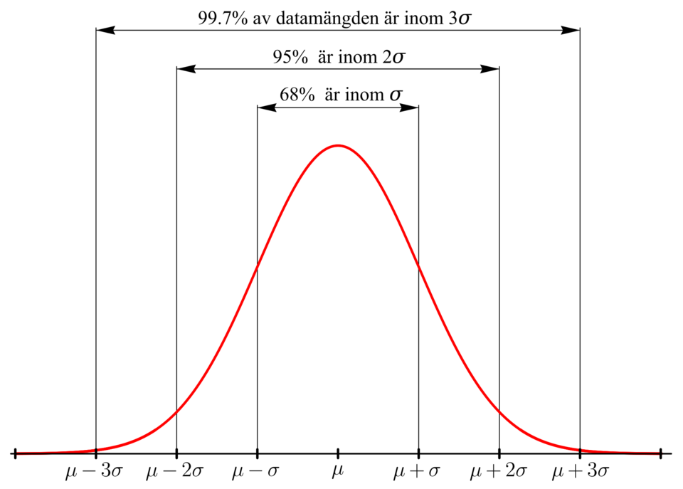
A labeled standard normal curve showing the proportions of data within 1, 2, and 3 standard deviations of the mean, illustrating the empirical rule. Source.

Key features include:

• About 68% of observations fall within 1 standard deviation of the mean (between μ − σ and μ + σ).

• About 95% fall within 2 standard deviations of the mean.

• About 99.7% fall within 3 standard deviations of the mean.

These predictable proportions allow students to identify unusual values, estimate ranges for typical observations, and compare different datasets using standardized units.

Interpreting Values in a Normal Distribution

Understanding the normal distribution helps students judge how extreme or typical a value is. Because the distribution is symmetric and centered at its mean, values far from the center become increasingly rare. A score that is several standard deviations away from the mean indicates an unusual observation. Recognizing these characteristics supports skill development in comparing datasets and evaluating the relative standing of observations.

When comparing two quantitative variables that each roughly follow a normal distribution, the parameters μ and σ allow for meaningful interpretation. For example, a distribution with a larger standard deviation will have values more widely dispersed, influencing the interpretation of what counts as typical or unexpected.

Using the Normal Model Appropriately

Students must remember that not all data follow a normal distribution. The normal model is appropriate only when the observed distribution is roughly symmetric, unimodal, and mound-shaped. Before applying concepts such as the empirical rule, students should visually assess the distribution using graphs like histograms or dotplots. A distribution that is skewed, multimodal, or contains strong outliers does not meet the assumptions of normality and will not follow predictable proportions around the mean.

Importance of the Normal Distribution in Statistical Reasoning

The normal distribution is foundational in statistical inference and probability. Its predictable structure allows for comparing distributions, interpreting standardized values, and assessing the likelihood of specific outcomes. Mastery of its characteristics supports deeper understanding of later topics, including z-scores, percentiles, and the use of technology to compute areas under normal curves.