
AP Syllabus focus:
‘Understand that t-distributions are used instead of normal distributions when estimating a test statistic with sample standard deviation s in place of the population standard deviation σ. More area in the tails of a t-distribution indicates higher probability for values further from the mean compared to a normal distribution. As degrees of freedom increase, t-distributions approach normal distributions.’
The t-distribution is essential in inference for means because it accounts for extra uncertainty introduced when using a sample standard deviation rather than a known population value.
The Role of t-Distributions in Statistical Inference
The t-distribution arises whenever a confidence interval or significance test for a population mean requires the use of the sample standard deviation, replacing the unknown population standard deviation. This substitution introduces additional variability, meaning the resulting sampling distribution must reflect wider possible outcomes than the normal model would allow.
Why t-Distributions Are Needed
When constructing intervals or performing tests about a population mean, conditions rarely allow the population standard deviation to be known. Because the statistic varies from sample to sample, using it inflates uncertainty. The t-distribution corrects for this by having heavier tails than the standard normal distribution. These heavier tails represent the increased chance of observing values far from the mean when estimating variability from sample data.
t-Distribution: A family of probability distributions used when estimating a population mean with unknown population standard deviation, characterized by heavier tails than the normal distribution.
This distribution is used specifically for inference involving a sample mean rather than a proportion, aligning directly with the situation described in the syllabus.
Understanding Degrees of Freedom
A central property of t-distributions is that they form a family, each identified by a parameter called degrees of freedom (df). In one-sample inference for a mean, the degrees of freedom equal n − 1, where n is the sample size. Degrees of freedom measure the amount of independent information available for estimating variability and help determine the spread of the corresponding t-distribution.
Degrees of Freedom (df): The number of independent values available for estimating a parameter, equal to n − 1 when computing a sample standard deviation.
Recognizing how degrees of freedom influence the distribution is crucial for selecting the correct critical value used in confidence intervals and significance tests.
Shape Characteristics of t-Distributions
All t-distributions share several structural features that support their use in inference about a population mean.
Heavier Tails and Their Implications
Compared with the normal distribution, t-distributions maintain the same overall symmetric, bell-shaped form but have more area in the tails.
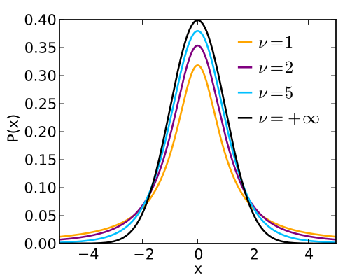
Probability density functions for Student’s t-distributions with various degrees of freedom compared with the standard normal distribution. Smaller degrees of freedom produce heavier tails, while larger degrees of freedom make the t-curve resemble the normal curve. The ν = 1 curve corresponds to the Cauchy distribution, which is an extra detail beyond the syllabus but reinforces tail behavior. Source.
This means they assign higher probability to extreme values. The syllabus highlights this characteristic because it directly reflects the extra uncertainty introduced when replacing σ with s. Heavier tails protect inference procedures from underestimating variability when sample sizes are small.
Normal distributions underestimate the likelihood of extreme deviations when the standard deviation must be estimated, making the t-distribution a safer model for small samples.
Convergence Toward the Normal Distribution
As sample size increases, the degrees of freedom also increase, and the t-distribution becomes narrower and more concentrated, gradually approaching the shape of the standard normal distribution. This occurs because larger samples produce more stable estimates of the population standard deviation, reducing the extra uncertainty that required the heavier-tailed distribution in the first place.
This transition explains why large-sample inference for means can sometimes use normal models, while small-sample inference must use t-distributions for accuracy.
Using t-Distributions for Critical Values
In confidence intervals and significance tests involving means, the critical value is taken from the appropriate t-distribution, determined by the degrees of freedom and the confidence level or tail probability.
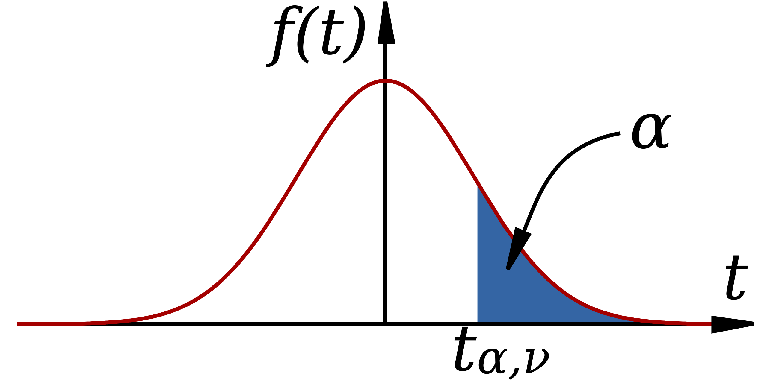
Diagram of a Student’s t-distribution showing a shaded tail beyond a critical value. The shaded region corresponds to a tail probability used to determine a critical value for inference. Labels such as tp,νt_{p,\nu}tp,ν, f(t)f(t)f(t), and p extend slightly beyond syllabus notation but support understanding of how cutoffs are selected. Source.
The heavy-tailed nature of t-distributions means these critical values are larger than those from the normal distribution when sample sizes are small, producing wider intervals and more conservative tests.
EQUATION
= Degrees of freedom, reflecting the sample size minus one
Because tail areas vary by degrees of freedom, students must select the correct distribution to ensure proper coverage probability for confidence intervals.
A key contrast is that larger critical values for small samples yield wider intervals, aligning with the increased uncertainty when estimating σ. As df grows, approaches the corresponding value from the standard normal distribution, reflecting decreasing uncertainty.
Summary of Key Properties
To understand and use t-distributions in the AP Statistics context, students must recognize the following features emphasized in the syllabus:
They are required when σ is unknown and s is used instead.
They have heavier tails than the normal distribution, reflecting higher probabilities of observing extreme values.
Their shape depends on degrees of freedom, forming a family of related distributions.
As degrees of freedom increase, t-distributions converge to the normal distribution.
They provide critical values necessary for constructing confidence intervals and conducting t-tests for means.
These properties ensure that inference procedures remain accurate and appropriately cautious when working with sample-based estimates of variability.
FAQ
With very small samples, the t-distribution becomes extremely heavy-tailed, meaning extreme values are far more likely than under the normal distribution.
This reflects the instability of the sample standard deviation when only one or two degrees of freedom are available.
Such small samples provide very weak information about population variability, so confidence intervals become extremely wide and critical values become very large.
The symmetry is a mathematical property of the statistic used to derive the t-distribution, not a reflection of the sample's distribution.
The t-distribution models the behaviour of the standardised sample mean, which remains symmetric around zero regardless of the sample's shape.
However, using the t-distribution is only appropriate when strong skewness or outliers are absent, especially in small samples.
When df is not an integer, tables typically round down to the nearest whole number to avoid understating uncertainty.
More refined tools, such as statistical software, interpolate between df values to obtain more precise critical values.
In AP Statistics contexts, using the nearest lower df is acceptable and slightly conservative.
Bootstrapping is flexible but conceptually more complex and computationally intensive.
The t-distribution provides a standardised, theory-based method that works well when conditions are met, especially with moderate sample sizes.
AP Statistics emphasises methods that are analytically transparent, easy to compute, and widely understood, making the t-distribution a natural choice.
Yes, provided the sample size is reasonably large or the sample data show no strong skewness or outliers.
Key considerations include:
• For n < 30, the sample should appear roughly symmetric and free of extreme points.
• For larger samples, the Central Limit Theorem helps stabilise the distribution of the sample mean.
Severely non-normal populations may still compromise t-based inference, particularly with small samples.
Practice Questions
Question 1 (1–3 marks)
A researcher is constructing a confidence interval for a population mean using a small random sample. The population standard deviation is unknown, so the researcher uses the sample standard deviation instead.
(a) State which distribution should be used for the interval.
(b) Explain why this distribution is appropriate in this situation.
Question 1
(a) 1 mark
• Correctly states that the t-distribution (Student’s t-distribution) should be used.
(b) 1–2 marks
• 1 mark for stating that the population standard deviation is unknown.
• 1 mark for explaining that using the sample standard deviation introduces extra variability, requiring a distribution with heavier tails (the t-distribution).
Total: 2–3 marks available
Question 2 (4–6 marks)
A student claims that as the sample size increases, the t-distribution becomes more similar to the standard normal distribution.
(a) Describe how the shape of the t-distribution changes as the degrees of freedom increase.
(b) Explain why the t-distribution has heavier tails than the normal distribution when the sample size is small.
(c) Discuss how these characteristics affect the critical values used in confidence intervals for small and large samples.
Question 2
(a) 1–2 marks
• 1 mark for stating that as degrees of freedom increase, the t-distribution becomes narrower or more concentrated.
• 1 mark for stating that it gradually approaches the shape of the standard normal distribution.
(b) 1–2 marks
• 1 mark for stating that heavier tails reflect increased uncertainty when estimating variability from a small sample.
• 1 mark for explaining that the sample standard deviation is less stable with small sample sizes, producing more extreme values.
(c) 2 marks
• 1 mark for stating that critical values from the t-distribution are larger for small samples because of heavier tails.
• 1 mark for stating that for large samples, critical values approach those from the normal distribution because uncertainty decreases.
Total: 4–6 marks available
