This section explains how to calculate a confidence interval for a population mean when the population standard deviation is unknown, using the t-distribution framework.

Calculating the Confidence Interval for a Mean

A confidence interval for a population mean provides a range of plausible values for the true mean, based on sample data. When the population standard deviation σ is unknown—which is almost always the case in applied statistics—students must rely on the sample standard deviation s, making the t-distribution the appropriate tool for inference.

Why the t-Distribution Is Used

Because substituting s for the unknown σ introduces extra variability, the resulting sampling distribution is wider than a normal distribution. The t-distribution accounts for this by having heavier tails, especially when sample sizes are small. As the sample size increases, the degrees of freedom grow, and the t-distribution approaches the normal distribution.

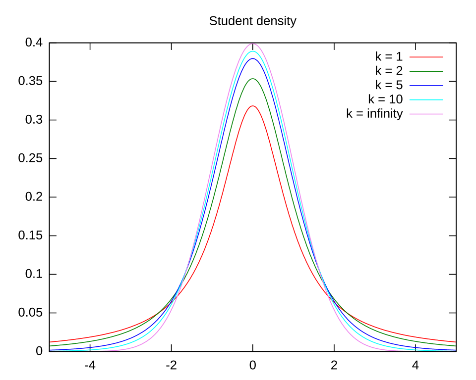
This plot compares Student’s t-distributions with the standard normal curve, illustrating heavier tails for low degrees of freedom and convergence toward normality as the degrees of freedom increase. Source.

Components of a Confidence Interval for a Mean

A one-sample t-interval requires three essential summary statistics from the sample: the sample mean, the sample standard deviation, and the sample size. These determine the standard error, which measures how much the sample mean is expected to vary across different random samples of equal size.

EQUATION

The critical value t* depends on the desired confidence level (commonly 90%, 95%, or 99%) and on degrees of freedom, which for a one-sample t-interval is n – 1. Technology or tables provide exact values.

Interpreting the Standard Error

The standard error of the sample mean describes the typical distance between the sample mean and the true population mean across repeated samples. When n is larger, the standard error decreases, leading to a narrower confidence interval.

EQUATION

This measure plays a direct role in determining the width of the confidence interval and the precision of the estimate.

Constructing the Interval Step by Step

To calculate the confidence interval for a population mean when σ is unknown, follow these structured steps:

• Identify sample statistics: Determine $\bar{x}$, $s$, and $n$ from the sample data.

• Compute the standard error: Use $s/\sqrt{n}$ to quantify variability in the estimate.

• Find the critical value t*:

  • Use the chosen confidence level.

  • Use n − 1 degrees of freedom.

• Calculate the margin of error: Multiply $t^*$ by the standard error.

• Construct the interval:

  • Lower bound: $\bar{x} - t^* \times \frac{s}{\sqrt{n}}$

  • Upper bound: $\bar{x} + t^* \times \frac{s}{\sqrt{n}}$

These steps provide a structured, repeatable process for any one-sample t-interval.

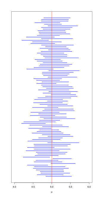
Each horizontal line represents a 95% confidence interval from a different random sample, illustrating the variation in interval endpoints and the long-run proportion of intervals that contain the true mean. Source.

Understanding the Margin of Error

The margin of error is the quantity added to and subtracted from the sample mean to create the confidence interval. It reflects uncertainty due to sampling variability.

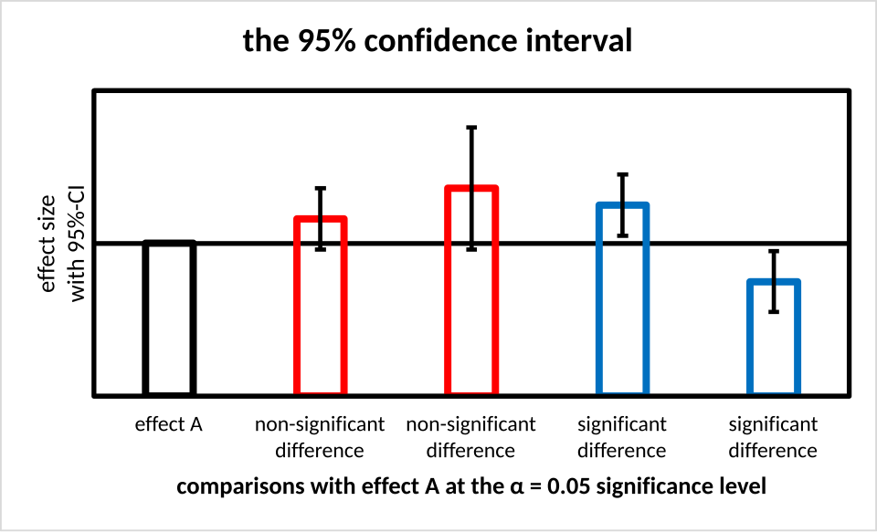
This bar chart displays sample means with their associated 95% confidence intervals, showing how the margin of error expands or contracts depending on variability and sample size. The figure also includes additional comparative context beyond the core syllabus requirement. Source.

• Larger t* values (associated with higher confidence levels or smaller sample sizes) increase the margin of error.

• A larger standard deviation also widens the interval.

• Increasing the sample size reduces the standard error and narrows the interval.

This relationship shows how design choices such as sample size affect precision.

Matched Pairs Situations

When dealing with matched pairs, such as before-and-after measurements on the same individuals, the analysis shifts the focus from individual observations to the set of paired differences.

For matched pairs:

• Compute the mean of the differences, $\bar{d}$.

• Compute the standard deviation of the differences, $s_d$.

• Let n be the number of paired differences.

• Use the same one-sample t-interval formula, replacing $\bar{x}$ with $\bar{d}$ and $s$ with $s_d$.

This method ensures that the interval estimates the population mean difference rather than the means of separate groups.

Interpreting the Confidence Interval

A correctly computed confidence interval describes a range of plausible values for the population mean based on the observed sample. The interpretation must always connect back to the context in which the data were collected. The interval’s width and location reflect sampling variability, sample size, and the chosen confidence level, helping students judge the reliability of estimates drawn from real-world data.