
AP Syllabus focus:
‘Independence: Data must be collected randomly, and if sampling without replacement, the sample size should be no more than 10% of the population. Normality: If the sample size is less than 30, the data should not show strong skewness or outliers; if skewed, a larger sample size is needed.’
Constructing a confidence interval for a population mean requires verifying key conditions that ensure the method’s validity. These conditions protect against biased inference and misleading conclusions.
Verifying Conditions for Confidence Intervals
Confidence intervals for population means rely on assumptions that support the use of the t-distribution and guarantee that the sample provides trustworthy information about the population. AP Statistics emphasizes two core requirements: independence and normality, each of which directly affects the reliability of the sampling distribution of the sample mean.
Independence Condition
The independence condition is essential because confidence interval formulas assume each observation contributes unique information. Violations of independence can artificially reduce variability, producing confidence intervals that are too narrow.
Independence: When the outcome of one observation does not influence the outcome of another, allowing each data point to contribute distinct information to the analysis.
To satisfy independence in practice, data must be randomly collected, either through a simple random sample or a randomized experiment.
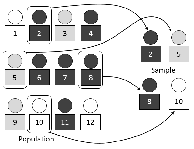
A visual representation of selecting a simple random sample from a larger population. Each individual has an equal chance of being chosen, illustrating the independence condition for inference. This image focuses on the random selection mechanism and does not depict the 10% condition explicitly. Source.
Random sampling ensures that the sample appropriately represents the population and that the natural variability in the data can be attributed to chance rather than systematic bias.
A second part of this condition applies when sampling without replacement. Because removing individuals from a finite population changes the probabilities for subsequent selections, AP Statistics uses the 10% condition to limit dependence introduced by sampling.
10% Condition: When sampling without replacement, the sample size must be no greater than 10% of the population to maintain approximate independence.
If a sample exceeds 10% of the population, the resulting confidence interval may underestimate variability, reducing its reliability. Therefore, confirming that the sampling method is random and that the sample is sufficiently small relative to the population is a critical early step.
Normality Condition
The normality condition concerns the shape of the population distribution and the sample size required for the t-procedures to remain valid. Because the t-distribution assumes that the sampling distribution of the sample mean is approximately normal, evidence of severe skewness or outliers can undermine inference accuracy.
Skewness: A measure of asymmetry in a distribution, where strong skewness indicates a long tail on one side that may distort the sampling distribution.
When the sample size is less than 30, AP Statistics requires checking that the sample does not exhibit strong skewness or outliers.
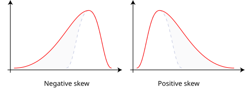
Diagrams illustrating negatively and positively skewed distributions. These shapes help students recognize when a sample’s distribution may violate the normality condition for constructing a t-interval. The curves focus only on skewness and do not show specific numerical values or test statistics. Source.
This inspection is typically performed using graphical methods such as dotplots, histograms, or boxplots.
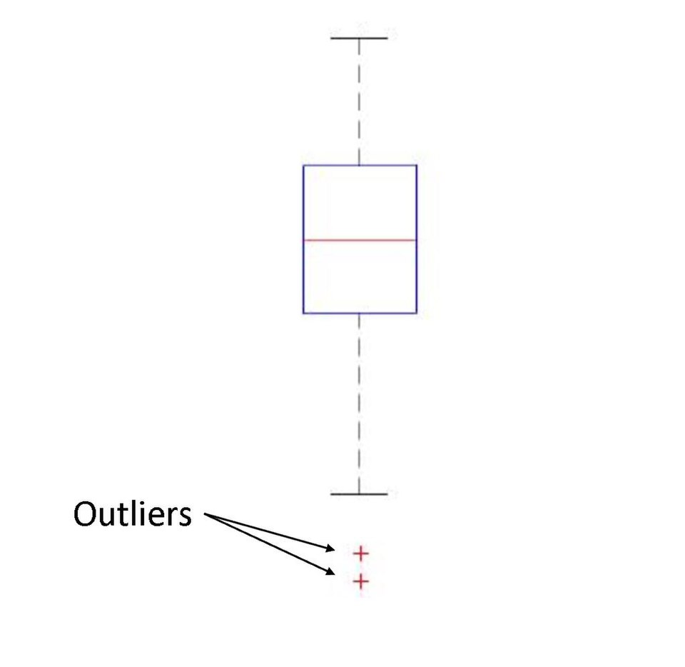
A boxplot displaying a distribution with outliers marked as separate points beyond the whiskers. This visualization highlights how outliers can be identified before deciding whether a t-interval is appropriate. The box and whiskers also show quartiles and overall spread, which goes slightly beyond the syllabus focus but provides helpful context for interpreting outliers. Source.
Data with pronounced abnormalities can cause the sampling distribution to deviate from normality, making the t-interval unreliable.
If the data appear skewed or contain outliers, a larger sample size is needed. Larger samples benefit from the Central Limit Theorem, which states that the sampling distribution of the sample mean becomes approximately normal as sample size increases, even if the population distribution itself is not normal. However, because the theorem does not guarantee normality for extremely small or highly skewed samples, verifying this condition is a necessary safeguard for valid inference.
The normality condition reinforces that a confidence interval should only be constructed when the sample provides a stable estimate of the population mean. Observations that are extreme or unevenly distributed weaken the assumptions behind the t-distribution and may widen the interval or distort its interpretive value.
Putting the Conditions Together
Before constructing a one-sample t-interval for a mean, both independence and normality must be verified. These conditions ensure that:
The sample is representative of the population.
The sampling distribution of the sample mean is approximately normal.
The margin of error accurately reflects expected variability.
A confidence interval is meaningful only when these foundational assumptions hold. Without independence, variability estimates become misleading. Without normality, the t-distribution no longer models the data effectively. Reviewing these conditions before proceeding with calculations ensures the resulting interval is statistically defensible and interpretable within the context of the research question.
FAQ
Skewness and outliers have the greatest influence on the shape of the sampling distribution when sample sizes are small, making them the key threats to validity for t-intervals.
Other features such as modality or slight irregularities usually have less effect on the robustness of the t-procedure, provided the distribution is not extreme.
The t-distribution is notably tolerant of mild non-normality, so only substantial departures, like heavy skew or extreme points, meaningfully compromise inference.
Technology allows for more detailed visualisation—histograms, boxplots, and normal probability plots—helping assess normality even when n is small.
When sample size increases, formal checking becomes less critical because the Central Limit Theorem provides protection against distributional irregularities.
However, for very small samples (n < 15), even technology cannot compensate for strongly skewed or heavily contaminated data, and t-intervals may be inappropriate.
In practice, independence should always be checked first because the validity of any statistical method depends on data representing the population without structural bias.
If independence fails, no amount of normality checking can salvage the inference, as the sample no longer reflects a valid random process.
Normality is then assessed to confirm that the sampling distribution of the mean supports using the t-distribution.
Acceptable evidence depends on the study design. Common indicators include:
• A clear description of simple random sampling
• Randomisation procedures in experiments
• Documentation of sampling frames or selection protocols
Indirect indicators, such as diversity of responses or evenly balanced sample characteristics, are not sufficient because they do not prove independence.
Acknowledge the limitation and assess the potential direction and magnitude of bias introduced.
Researchers may:
• Use wider confidence intervals to reflect greater uncertainty
• Refrain from formal inference and limit conclusions to descriptive summaries
• Conduct sensitivity analyses, such as comparing subgroups, to evaluate plausibility of independence
Confidence intervals constructed under doubtful independence should be interpreted with caution and explicitly flagged as potentially unreliable.
Practice Questions
Question 1 (1–3 marks)
A researcher collects a random sample of 18 observations from a population in order to construct a confidence interval for the population mean. A dotplot of the data shows several values clustered near the centre and one noticeably extreme value far to the right.
(a) State whether the normality condition for constructing a one-sample t-interval is likely to be met.
(b) Briefly justify your answer.
Question 1 (3 marks total)
(a) Indicates that the normality condition is likely not met due to the presence of an extreme value.
1 mark
(b) Explains that with a sample size less than 30, strong skewness or outliers violate the normality assumption required for a t-interval.
1–2 marks
1 mark for referencing the impact of the outlier on normality.
1 additional mark for correctly linking this to the small sample size requirement.
Question 2 (4–6 marks)
A school wishes to estimate the average number of hours students spend revising per week. They take a random sample of 26 students from the school population.
(a) Explain why the independence condition must be checked before constructing a confidence interval for the mean revision time.
(b) The school has 1,200 students. Determine whether the 10% condition is satisfied and explain its importance.
(c) A histogram of the sample data shows a moderate right skew but no clear outliers. Discuss whether the normality condition is met and whether it would be appropriate to use a one-sample t-interval.
Question 2 (6 marks total)
(a) States that independence ensures each observation provides unique information and prevents underestimation of variability.
1–2 marks
1 mark for referencing independence.
1 mark for explaining why it matters for confidence intervals.
(b) Correctly checks the 10% condition: 26 is less than 10% of 1,200 (which is 120), so the condition is satisfied.
1–2 marks
1 mark for correct comparison.
1 mark for explaining that this maintains approximate independence when sampling without replacement.
(c) Notes that moderate skew without outliers is acceptable with a sample size above 30 being preferred, but with n = 26 the t-interval may still be reasonable if skewness is not strong.
2–3 marks
1 mark for discussing skewness.
1 mark for referencing appropriateness of t-procedures.
1 mark for correct interpretation of the sample size relative to the condition.
