This section explains how a t-statistic is computed for hypothesis testing about a population mean when the population standard deviation is unknown, highlighting why each component matters.

Calculating the Test Statistic for a Population Mean

The t-statistic is the foundational numerical measure used in a one-sample t-test, quantifying how far the observed sample mean lies from the hypothesized population mean in standardized units. Because the population standard deviation is typically unknown in real research, the sample standard deviation replaces it, introducing additional variability. This adjustment leads to the use of the t-distribution, which is wider and has heavier tails than the normal distribution, especially with small sample sizes.

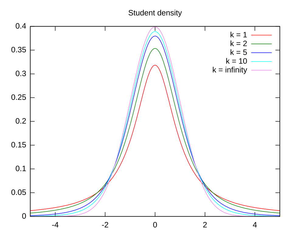
This set of t-distribution curves illustrates how heavier tails arise at low degrees of freedom and how the curves converge toward the normal distribution as sample size increases. Source.

The test statistic allows researchers to evaluate whether the observed data are consistent with the null hypothesis or provide evidence for the alternative hypothesis.

Understanding the Components of the t-Statistic

The test statistic compares the observed sample mean to the hypothesized mean, adjusted for expected sampling variability. To perform this calculation, several core quantities must be used carefully and interpreted correctly.

The sample mean summarizes the center of the collected data and is the key point of comparison against the hypothesized mean.

This hypothesized value establishes the benchmark for assessing whether the sample provides evidence of a difference.

Because $s$ replaces the unknown population standard deviation in inference procedures, it adds uncertainty reflected by the t-distribution.

Sample size influences the precision of the estimate and determines the degrees of freedom, which affect the shape of the t-distribution used to determine probabilities associated with the test statistic.

A clear understanding of these components ensures that the calculated test statistic accurately reflects the strength of evidence in the data.

The Formula for the Test Statistic

The AP Statistics syllabus requires mastery of the formula used to compute the t-statistic in a one-sample mean test. This calculation standardizes the difference between the sample mean and the hypothesized mean by dividing by the standard error, which represents the expected variation of sample means.

EQUATION

This formula yields a value measured in standard error units, indicating how unusual the sample result would be if the null hypothesis were true.

After calculating the statistic, it is interpreted using the t-distribution with $n - 1$ degrees of freedom, which adjusts for the estimation of variability using sample data rather than known population parameters.

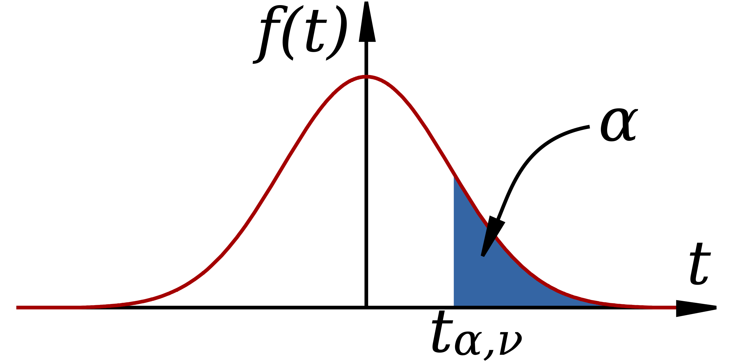
This diagram highlights a critical value on a t-distribution curve, showing how calculated t-statistics are interpreted relative to degrees of freedom and associated tail areas. Source.

Why the t-Distribution Is Required

When the population standard deviation is unknown—almost always in practical settings—replacing it with the sample standard deviation introduces additional variability. The t-distribution compensates for this by stretching its tails, increasing the probability of more extreme values. As sample size grows, the sample standard deviation becomes a more stable estimate, causing the t-distribution to closely approximate the normal distribution. This behavior ensures that the test statistic is assessed using an appropriate reference distribution that accounts for uncertainty inherent in the data.

Calculating the Test Statistic for Matched Pairs

The syllabus also specifies that matched-pairs designs require computing differences within each pair before applying the same one-sample t-test procedure. This reframing converts the paired data into a single quantitative variable: the set of differences.

Once these differences are computed, the same components used in the one-sample t-test apply, but now to the mean and standard deviation of the differences. This ensures that the analysis targets the change within subjects or matched units, rather than comparing paired observations independently.

In matched-pairs settings, the test statistic evaluates whether the mean difference in the population is equal to the hypothesized value specified in the null hypothesis. The procedure maintains the same form as the one-sample mean test but uses the difference statistics instead of original measurements.

Interpreting the Role of Degrees of Freedom

The degrees of freedom, calculated as $n - 1$, reflect the number of independent pieces of information available to estimate the population standard deviation. This affects the exact shape of the t-distribution used to determine probabilities associated with the test statistic. Smaller samples yield fewer degrees of freedom, widening the distribution and requiring stronger evidence (a larger absolute test statistic) to question the null hypothesis. As sample size increases, the distribution narrows, improving the precision of the test.

Structural Overview of the Calculation Process

To ensure clear understanding and strong procedural habits, the essential components of calculating the test statistic include:

• Identifying the sample mean and hypothesized mean for comparison.

• Determining the sample standard deviation to estimate population variability.

• Computing the standard error using $s/\sqrt{n}$.

• Standardizing the difference between $\bar{x}$ and $\mu_0$ using the t-statistic formula.

• Referring to the correct t-distribution based on degrees of freedom.

• Applying the same structure to matched-pairs data using differences.

Each step contributes to producing a valid and interpretable test statistic that aligns with the AP Statistics inference framework.