
AP Syllabus focus:
‘Chi-square distributions are right-skewed and only take positive values, with skewness decreasing as degrees of freedom increase. Expected counts in categorical data are derived from sample size multiplied by the probability of each category under the null hypothesis. The chi-square statistic quantifies the discrepancy between observed and expected counts, providing a measure of how far the observed data deviate from what was expected under the null hypothesis.’
Understanding Chi-Square Distributions
Chi-square distributions form the foundation of inference procedures for categorical data, helping quantify how far observed counts differ from expected values under a hypothesized model.
Characteristics of Chi-Square Distributions
Chi-square distributions have several essential properties that shape how statistical inference is conducted using the chi-square statistic.
They take only positive values because they are based on squared differences between observed and expected counts.
They are right-skewed, meaning most values cluster near zero with a long tail extending to the right.
Skewness decreases as degrees of freedom increase, making the distribution approach a more symmetric shape as categories or complexity grow.
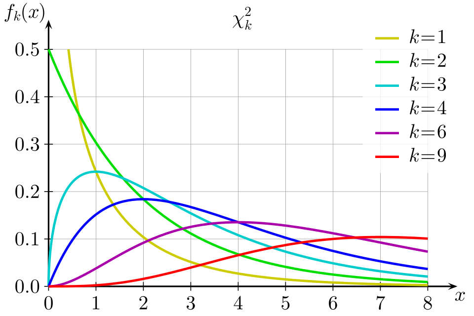
Chi-square probability density functions for several degrees of freedom, illustrating right skew and decreasing skewness as degrees of freedom increase. The printed formula in the corner exceeds AP requirements and can be ignored. Source.
The term degrees of freedom is used frequently in chi-square procedures and represents the number of independent pieces of information available for estimating variation.
Degrees of Freedom: The number of independent categories minus one, determining the shape of the chi-square distribution.
As the degrees of freedom rise, the center of the distribution shifts rightward, reflecting greater expected variability when more categories are present.
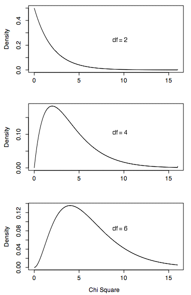
A comparison of chi-square distributions for different degrees of freedom, showing how the peak shifts to the right and becomes less skewed as degrees of freedom increase. Source
Understanding Expected Counts
Expected counts represent what should be observed in each category if the null hypothesis accurately describes the population. Under the null model, they reflect theoretical proportions applied to the sample size.
Expected Count: The predicted frequency in a category, computed by multiplying the total sample size by the hypothesized probability of that category.
Expected counts serve as a baseline for evaluating how surprising the actual data appear. When observed counts differ only slightly from expectations, chance alone may explain the discrepancies. Substantial differences, however, may suggest that the null model does not adequately describe the population.
A formulaic representation of expected counts reinforces this conceptual foundation.
EQUATION
= Total sample size
= Null proportion for category
Understanding expected counts is crucial because inaccurate or improperly calculated expectations can distort the chi-square statistic and invalidate conclusions.
The Chi-Square Statistic as a Measure of Discrepancy
The chi-square statistic quantifies the distance between observed and expected values, taking the squared differences and weighting them relative to the expected count. This design ensures that the contribution of each category reflects both the size of the deviation and the expected magnitude.
Chi-Square Statistic: A numerical measure representing the aggregated squared deviations between observed and expected counts, scaled by expected counts.
Its structure ensures that categories with very small expected counts do not disproportionately influence results and that extreme deviations receive greater weight.
EQUATION
= Observed count in a category
= Expected count in a category
Because each term of the statistic involves squared differences and positive expected counts, the resulting chi-square value must always be nonnegative, aligning naturally with the right-skew of the chi-square distribution.
Why Chi-Square Distributions Matter in Inference
Chi-square distributions allow researchers to judge whether the chi-square statistic is unusually large relative to what would be expected by chance. Their right-skewed form means that high values indicate outcomes that are improbable if the null hypothesis were true.
Key conceptual points include:
Small chi-square values suggest observed data closely follow expectations.
Larger values signal increasing discrepancy and potential evidence against the null hypothesis.
The appropriate chi-square distribution depends entirely on the degrees of freedom associated with the model.
This connection between the discrepancy measure and the distributional shape is central to categorical inference. By understanding how chi-square distributions behave, why expected counts are computed from null proportions, and how the chi-square statistic summarizes deviation, students build the conceptual foundation for applying chi-square tests responsibly across categorical scenarios.
FAQ
As degrees of freedom increase, the distribution is formed from the sum of more independent squared standard normal variables. With more components contributing, the variability balances out, producing a shape that moves closer to a normal distribution.
This shift also occurs because the centre of the distribution increases, reducing the influence of the long right tail relative to the overall spread.
The centre (mean) of a chi-square distribution equals the degrees of freedom. Because the statistic reflects accumulated squared deviations, more categories naturally produce a higher average chi-square value.
This does not represent a typical or likely observed chi-square statistic; rather, it reflects the theoretical long-run average if repeated random samples were taken.
The chi-square statistic is always positive because it sums squared quantities, giving it a boundary at zero. Values near zero are much more likely than large deviations.
Symmetry is impossible because large positive deviations are unbounded, but negative deviations cannot exist. This imbalance produces the characteristic right-skew.
As degrees of freedom rise, the variance increases, meaning the possible chi-square values spread out over a wider range.
However, the relative spread decreases. The standardised shape becomes more concentrated around the centre, which is why the curve appears smoother and less skewed even as its numerical range expands.
Using squared deviations ensures all contributions are positive and magnifies larger discrepancies, which is essential when assessing how far observed counts are from expected ones.
Squaring also aligns the statistic with theoretical probability models based on sums of squared normal variables, allowing chi-square distributions to serve as the appropriate reference distributions for inference.
Practice Questions
Question 1 (1–3 marks)
A researcher analyses categorical data and notes that the chi-square distribution used for the test is right-skewed and takes only positive values.
(a) Explain why the chi-square statistic can never be negative. (1 mark)
(b) State how increasing the degrees of freedom affects the shape of the chi-square distribution. (1–2 marks)
Question 1
(a) 1 mark
• The chi-square statistic involves squared differences between observed and expected counts, so the value cannot be negative.
(b) 1–2 marks
• 1 mark: States that the distribution becomes less skewed / more symmetric as degrees of freedom increase.
• 1 mark: Notes that the distribution shifts to the right / spreads out more with increasing degrees of freedom.
Question 2 (4–6 marks)
A study investigates whether a theoretical model accurately predicts the distribution of outcomes across five categories. The expected counts are calculated using the sample size multiplied by the probabilities specified under the null hypothesis.
(a) Define an expected count in this context. (1 mark)
(b) Describe how large discrepancies between observed and expected counts will affect the value of the chi-square statistic. (1–2 marks)
(c) Explain why the chi-square distribution is appropriate for modelling the test statistic in this scenario, referring to its key properties. (2–3 marks)
Question 2
(a) 1 mark
• An expected count is the predicted frequency in a category based on the sample size and the null hypothesis probabilities.
(b) 1–2 marks
• 1 mark: States that larger discrepancies lead to larger chi-square contributions.
• 1 mark: Acknowledges that this increases the overall chi-square statistic because deviations are squared and divided by the expected count.
(c) 2–3 marks
• 1 mark: Mentions that the chi-square statistic is always positive, aligning with the chi-square distribution’s domain.
• 1 mark: States that the distribution is right-skewed, especially for small degrees of freedom.
• 1 mark: Notes that the degrees of freedom depend on the number of categories, making the chi-square distribution suitable for categorical comparisons.
