
OCR Specification focus:
‘Plot V against I to obtain internal resistance and e.m.f. from gradient and intercept.’
In analysing electrical sources, graphical methods provide a powerful way to determine both internal resistance and electromotive force (e.m.f.). By plotting measured values of terminal potential difference (V) against current (I), students can extract these quantities accurately while visually understanding how internal resistance affects circuit performance.
Understanding Internal Resistance and Electromotive Force
A source of e.m.f., such as a cell or power supply, delivers energy to charge carriers. However, real sources have internal resistance (r), causing energy losses within the source itself. As current increases, some of the supplied energy is dissipated as heat inside the source, reducing the terminal voltage available to the external circuit.
Electromotive Force (E or e.m.f.): The total energy supplied per unit charge by the source when no current flows (unit: volt, V).
Internal Resistance (r): The effective resistance within a power source that causes energy losses as current flows (unit: ohm, Ω).
This internal resistance leads to a difference between the e.m.f. and the terminal potential difference (V). The relationship between them can be expressed through a key equation.
EQUATION
—-----------------------------------------------------------------
Internal Resistance Equation (E = V + Ir)
E = electromotive force (V)
V = terminal potential difference across the external circuit (V)
I = current in the circuit (A)
r = internal resistance of the source (Ω)
—-----------------------------------------------------------------
When no current flows, I=0I = 0I=0, so the terminal voltage equals the e.m.f. As current increases, IrIrIr (known as the lost volts) rises, reducing V below E.
The Principle of Graphical Analysis
Graphical analysis offers a visual and quantitative method to determine E and r. It uses experimentally measured pairs of V and I values plotted on a graph to reveal their linear relationship.
When rearranged, the internal resistance equation becomes:
EQUATION
—-----------------------------------------------------------------
Rearranged Linear Form (V = E – Ir)
V = terminal potential difference (V)
E = electromotive force (V)
I = current (A)
r = internal resistance (Ω)
—-----------------------------------------------------------------
This equation is of the form y = c + mx, where:
y corresponds to V (the dependent variable),
x corresponds to I (the independent variable),
c is the y-intercept (E),
m is the gradient (-r).
Therefore, plotting V on the y-axis and I on the x-axis produces a straight-line graph with:
y-intercept = E (electromotive force)
gradient = –r (negative of internal resistance)
This graphical approach is particularly valuable in experimental physics, where trends and relationships can be observed even when measurements include uncertainty.
Plotting V against I produces a straight line; the y-intercept equals the emf E and the gradient equals −r.
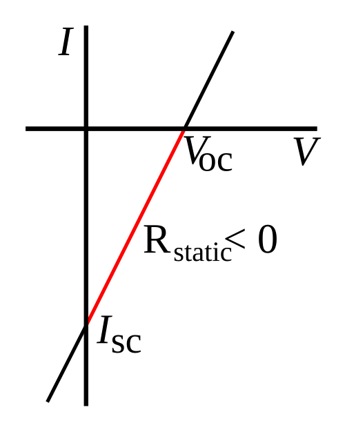
Current–voltage characteristic of a cell modelled by an ideal source in series with internal resistance. The open-circuit voltage VocV_\text{oc}Voc is the intercept at I=0I=0I=0, and the short-circuit current Isc=Voc/rI_\text{sc}=V_\text{oc}/rIsc=Voc/r is the intercept at V=0V=0V=0. The straight-line form underpins the graphical method where gradient = −r and intercept = E. The image text includes “negative static resistance,” referring only to the source’s polarity convention. Source.
Experimental Setup and Data Collection
When carrying out this analysis in a laboratory environment, the circuit typically includes:
a cell or power supply (the e.m.f. source),
an ammeter to measure current,
a voltmeter to measure terminal potential difference across the source,
a variable resistor to adjust current and obtain different readings.
The experiment proceeds as follows:
Connect the circuit so that current passes through both the cell and the variable resistor.
Vary the resistance to obtain several pairs of current (I) and voltage (V) readings.
Record measurements over a range of currents, ensuring readings are evenly spaced and within the safe operating range of the cell.
Plot V against I using the recorded data.
Good experimental practice includes minimising systematic error by ensuring accurate voltmeter calibration and by allowing the cell to cool between readings to avoid thermal changes affecting internal resistance.
Interpreting the V–I Graph
Once plotted, the V–I graph should form a straight descending line. The key interpretation steps are:
The y-intercept (V when I = 0) gives the e.m.f. (E) — this is the voltage of the source when no current flows.
The gradient (ΔV / ΔI) equals –r, allowing internal resistance to be calculated as the negative of the slope.
By using the best-fit line, rather than individual points, random measurement errors are minimised and more reliable estimates for E and r are achieved.
When the line deviates from linearity, it may indicate changes in internal temperature, nonlinear source behaviour, or measurement error. Such effects highlight the importance of experimental control.
Accuracy, Precision, and Uncertainties
Graphical analysis not only determines key quantities but also visualises experimental uncertainty:
Scatter of points around the best-fit line reflects random error.
Gradient uncertainty can be estimated by drawing lines of maximum and minimum slope consistent with the data.
Intercept uncertainty provides an estimate for the possible range of e.m.f. values.
Students should always record measurements to an appropriate number of significant figures and include error bars when plotting graphs.
Label axes with V (y-axis) and I (x-axis), draw a best-fit straight line, and read off intercept E and gradient −r with appropriate units.

Straight-line V–I graph with a clean best-fit line and labelled axes. Although it depicts an ohmic resistor (so gradient = R), the graphing conventions are identical to those for the V–I analysis of a cell, where intercept gives E and negative gradient gives r. The image includes extra resistor-specific labels beyond the OCR syllabus. Source.
Common sources of uncertainty include:
Voltmeter accuracy and internal resistance.
Ammeter calibration drift.
Heating effects changing internal resistance.
Contact resistance at terminals or leads.
Significance of Graphical Analysis in Physics
Graphical methods illustrate the underlying physics of electrical energy transfer. As current increases, internal resistance causes more energy to dissipate as heat, reducing terminal voltage. The linear relationship confirms Ohmic behaviour within the operating limits of the source.
Moreover, the graphical determination of e.m.f. and internal resistance is not merely a practical exercise; it reinforces key theoretical principles:
Energy conservation within the circuit.
The distinction between e.m.f. (total energy per charge supplied) and terminal potential difference (useful energy per charge delivered to the external circuit).
The effect of internal resistance as a limitation on energy efficiency.
This analysis aligns directly with the OCR specification focus — students are expected to plot V against I and determine e.m.f. and internal resistance from the graph’s intercept and gradient, respectively.
Practice Questions
Question 1 (2 marks)
A student connects a cell of e.m.f. 1.5 V and internal resistance r in series with a resistor. When the current in the circuit is 0.30 A, the terminal potential difference across the cell is 1.35 V.
(a) Calculate the internal resistance of the cell.
Mark Scheme for Question 1
Correct use of equation E = V + Ir (1 mark)
Substitution: 1.5 = 1.35 + (0.30 × r), leading to r = 0.50 Ω (1 mark)
Question 2 (5 marks)
A student is investigating the internal resistance and e.m.f. of a cell using the circuit shown below. The student measures the terminal potential difference V for several values of current I and plots a graph of V against I. The graph is a straight line with an intercept at 1.6 V and a gradient of –0.40 Ω.
(a) State what the intercept on the V-axis represents. (1 mark)
(b) State what the gradient of the line represents. (1 mark)
(c) Using the information from the graph, write the equation that links V and I for this cell. (1 mark)
(d) Explain why it is important to take readings quickly when performing this experiment. (2 marks)
Mark Scheme for Question 2
(a) Intercept represents the e.m.f. of the cell (1 mark)
(b) Gradient represents the negative of the internal resistance (–r) (1 mark)
(c) V = 1.6 – 0.40I (1 mark)
(d)
As current flows, the cell warms up (1 mark)
This causes the internal resistance to change with temperature, affecting accuracy (1 mark)
FAQ
The V–I graph for a cell remains a straight line because the internal resistance of the cell behaves approximately as a fixed, ohmic resistance under normal operating conditions.
In this range, the relationship between terminal voltage and current (V = E – Ir) is linear. Curved graphs appear only if the internal resistance changes significantly, such as when the cell heats up or undergoes chemical depletion.
As temperature increases, the ions in the electrolyte move more freely, reducing the internal resistance temporarily.
However, prolonged current flow can cause polarisation or chemical changes that increase resistance again.
To minimise these effects:
Allow the cell to cool between readings.
Avoid drawing large currents for extended periods.
Take measurements promptly to keep conditions stable.
The voltmeter must measure the terminal potential difference, which excludes the voltage drop across external components.
Connecting it directly across the cell ensures it records only the potential difference available from the source. If connected elsewhere, the reading would include other circuit losses, leading to an incorrect calculation of e.m.f. and internal resistance.
Typical sources of error include:
Inaccurate current or voltage measurements due to meter resolution limits.
Poor electrical contacts or corroded terminals increasing resistance.
Temperature rise in the cell affecting internal resistance.
Parallax errors when reading analogue instruments.
Using digital meters, secure connections, and consistent measurement timing helps reduce these errors.
Uncertainties are typically determined using lines of best fit and worst acceptable fit.
Draw a best-fit line through the data points.
Then sketch two extreme lines that still pass through all error bars.
The variation in gradient gives the uncertainty in internal resistance (r).
The range of intercepts gives the uncertainty in e.m.f. (E).
This graphical method visually represents measurement reliability and helps quantify confidence in the results.
