
OCR Specification focus:
‘Recognise exponential decay graphs and the constant-ratio property for successive equal time intervals.’
Exponential decay in capacitor discharge appears frequently in A-Level Physics. Understanding its graphical behaviour and characteristic constant-ratio property is essential for analysing real capacitor–resistor circuits confidently and accurately.
Exponential Decay in Capacitor–Resistor Circuits
When a capacitor discharges through a resistor, the physical quantities of charge, current, and potential difference decrease over time in a distinctive manner described as exponential decay. This behaviour arises because the rate at which these quantities fall is always proportional to their instantaneous values. As the capacitor empties, the driving p.d. across the resistor diminishes, causing smaller and smaller decreases per unit time. The OCR specification emphasises the ability to recognise exponential decay graphs and the constant-ratio property for successive equal time intervals, so graphical interpretation is a core requirement.
Key Characteristics of Exponential Decay
Exponential decay exhibits several unique graphical features that allow students to identify it with confidence:
A smooth, continuous curve declining steeply at first and flattening progressively.
A gradient that becomes steadily less negative as time increases.
No sharp corners, discontinuities, or sudden slope changes.
A decreasing quantity that never reaches zero within finite time but approaches it asymptotically.
These features hold regardless of whether the vertical axis represents charge, current, or potential difference, because all three follow a similar exponential form during discharge.
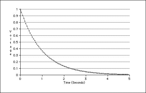
Graph of a capacitor’s voltage or charge decreasing exponentially with time during discharge. The curve is steep at first and gradually flattens. This characteristic non-linear decay matches the expected behaviour for charge, current, or potential difference in an RC discharge. Source.
The Mathematical Form of Exponential Decay
In a capacitor–resistor system, exponential decay is typically expressed using the general form:
EQUATION
—-----------------------------------------------------------------
Exponential Decay (x(t)) = x₀ e^(−t/RC)
x(t) = Value of the decaying quantity at time t (unit varies)
x₀ = Initial value of the quantity at t = 0 (unit varies)
t = Time (s)
R = Resistance (Ω)
C = Capacitance (F)
—-----------------------------------------------------------------
Between any two such equations, the curve describing the behaviour follows the same exponential trend. Although the mathematical form is important, at this stage the specification focuses more strongly on recognition and interpretation of exponential decay properties than on manipulation or calculation.
This model explains why exponential graphs are distinctively curved: each small time step reduces the quantity by a fraction rather than by a fixed amount.
Recognising Exponential Decay Graphs
Graph recognition is frequently examined, and students should be able to identify exponential decay even when the axes represent unusual or less familiar variables. When inspecting graphs:
Look for a rapid initial drop followed by a gradual flattening.
Check that the curve gets closer to the time axis but never crosses it.
Observe that equal time intervals produce proportional rather than identical decreases.
Confirm that negative values or sudden jumps are absent, as these do not occur in physical capacitor discharge.
In typical physics contexts, exponential decay is visualised for charge on the capacitor, current in the circuit, or potential difference across the capacitor or resistor. Despite these being different physical quantities, their curves share identical shapes because each depends on the same underlying discharge process.
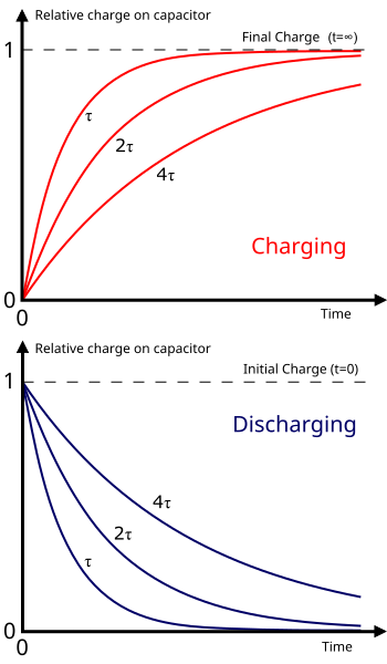
Graphs of relative charge during capacitor charging and discharging, plotted with multiples of the time constant τ. The exponential discharge curve demonstrates the same fractional change over equal time intervals. The charging curve provides additional context not required by the subsubtopic but helpful for comparison. Source.
The Constant-Ratio Property
A defining feature of exponential decay, highlighted explicitly in the OCR specification, is the constant-ratio property, which states that for any quantity undergoing exponential decay, the ratio of its value at the end of one equal time interval to its value at the beginning of the interval remains constant. In other words, successive drops follow a consistent fractional pattern.
Constant-Ratio Property: The characteristic behaviour of exponential decay in which the ratio of the quantity’s value after an equal time interval to its starting value remains constant.
This is profoundly different from linear decay, where the quantity decreases by equal amounts over equal time periods. In exponential decay, decreases become progressively smaller, yet follow a predictable pattern. This property provides a reliable method for identifying exponential relationships in experimental data, even when noise or measurement uncertainty is present.
Because capacitor discharge follows e−t/RCe^{-t/RC}e−t/RC, the constant-ratio property emerges directly from the exponential term. The ratio depends on the value of RC, the time constant, but once this value is fixed, the ratio remains the same for every equal time interval.
Interpreting the Constant-Ratio Property on Graphs
Students should be able to infer the presence of exponential decay by visually recognising this ratio behaviour. While reading from a graph:
Select equal time intervals along the horizontal axis.
Compare the vertical-axis readings at the start and end of each interval.
Check whether the ratios (not the differences) are consistent.
If they are, the graph almost certainly represents exponential decay.
A normal sentence is placed here to ensure that no definition or equation blocks sit immediately next to each other.
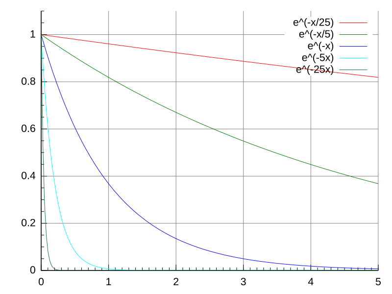
Multiple exponential decay curves illustrating how different decay constants affect the rate of decline. Each curve demonstrates the same fractional drop over equal time intervals, embodying the constant-ratio property. Although general, the behaviour directly matches that of capacitor discharge when the axes represent time and charge, voltage, or current. Source.
Implications for Capacitor Behaviour
The constant-ratio property helps explain several physical observations in capacitor discharge:
The current drops rapidly at first because the capacitor initially has a large potential difference.
As the voltage falls, the driving force for current weakens, producing smaller current decreases with time.
Because the decay is always proportional, the curve never levels out completely, though it becomes extremely close to zero.
These characteristics make exponential decay essential for understanding timing behaviour in electronic circuits, including filters, timing circuits, and sensing devices. Exponential decay is therefore a foundational concept that underpins more advanced circuit analysis and practical applications involving capacitors.
Practice Questions
Question 1 (2 marks)
A student examines a graph showing the discharge of a capacitor through a resistor. Describe two features of the graph that indicate the quantity is undergoing exponential decay.
Question 1 (2 marks)
Award 1 mark for each correct feature, up to 2 marks.
• The graph falls steeply at first and then gradually flattens as time increases. (1)
• The quantity approaches zero asymptotically and never reaches zero in a finite time. (1)
• The decreases in value get progressively smaller over time, indicating non-linear decay. (1)
Question 2 (5 marks)
A capacitor discharges through a resistor. Explain what is meant by the constant-ratio property of exponential decay and describe how a student could use a discharge graph to confirm that the capacitor’s behaviour follows exponential decay. In your answer, refer to the changes in the quantity over equal time intervals and how these relate to the RC time constant.
Question 2 (5 marks)
Award marks for the following points:
• Statement that exponential decay has a constant-ratio property: over equal time intervals, the quantity decreases by the same fraction, not the same amount. (1)
• Explanation that this fractional decrease remains constant throughout the discharge. (1)
• Student should take readings of the quantity (e.g., voltage, current, or charge) at equal time intervals from the graph. (1)
• The student should calculate the ratio of values at the end and start of each equal interval. (1)
• If these ratios are the same (or approximately the same within experimental variation), this confirms exponential decay. (1)
• Reference to how this behaviour is linked to the RC time constant controlling the rate of decay. (1)
FAQ
Look for the overall trend rather than individual fluctuating points. If the data roughly follows a smooth curve that flattens with time, it is likely exponential.
A useful approach is to calculate ratios across several equal time intervals and take an average.
• If the ratios cluster around a consistent value, the behaviour is exponential.
• If ratios vary randomly with no pattern, the data may be too noisy or not exponential.
Mathematically, exponential decay approaches zero asymptotically, meaning the quantity decreases forever without becoming exactly zero.
In practice, the capacitor appears discharged because the remaining charge produces a voltage too small to drive measurable current. Real components also have leakage paths that remove the final residual charge.
Several non-ideal factors influence real behaviour:
• Internal leakage resistance inside the capacitor
• Parasitic resistances and inductances in wires or connections
• Temperature-dependent changes in resistance
• Dielectric absorption causing charge to reappear briefly after discharge
These effects distort the perfect exponential model but usually become significant only in precise measurements.
Yes, if the product RC (the time constant) is the same for both circuits.
For example:
• A small capacitor with a large resistor
• A large capacitor with a small resistor
Both combinations can produce the same time constant, leading to identical decay shapes, even though the individual component values differ.
Visual inspection can be misleading, especially with limited data points or low-resolution graphs.
The constant-ratio method uses numerical comparison of values, reducing subjective interpretation.
• It works even when the graph covers only a small section of the decay.
• It can distinguish exponential decay from other curve types that look similar early on, such as power-law decay.
