
OCR Specification focus:
‘Apply equations of motion for constant acceleration, including free-fall without air resistance: v=u+at, s=ut+½at², v²=u²+2as.’
The SUVAT equations describe motion under constant acceleration and are essential for analysing objects moving in a straight line, including freely falling bodies without air resistance.
The Concept of Constant Acceleration
When an object experiences a constant acceleration, its rate of change of velocity remains the same throughout the motion. This condition allows us to derive relationships between displacement, velocity, acceleration, and time. These relationships are expressed through the SUVAT equations, where each letter represents a key physical quantity.
Displacement (s): The total distance moved in a specific direction; it is a vector quantity measured in metres (m).
Velocity (v): The rate of change of displacement; it has both magnitude and direction and is measured in metres per second (m s⁻¹).
Acceleration (a): The rate of change of velocity per unit time, measured in metres per second squared (m s⁻²).
In uniform acceleration, these quantities are directly linked. The motion may involve an object speeding up, slowing down, or changing direction, provided that acceleration remains constant.
The SUVAT Quantities
The term SUVAT represents the five main variables involved in equations of motion:
s – Displacement (m)
u – Initial velocity (m s⁻¹)
v – Final velocity (m s⁻¹)
a – Constant acceleration (m s⁻²)
t – Time (s)
These equations apply only when acceleration is constant and motion occurs along a straight line.
The Equations of Motion for Constant Acceleration
The following three core equations form the foundation of constant acceleration analysis. Each equation relates different combinations of the SUVAT variables.
EQUATION
—-----------------------------------------------------------------
First Equation of Motion (v–t relationship)
v = u + at
v = Final velocity (m s⁻¹)
u = Initial velocity (m s⁻¹)
a = Constant acceleration (m s⁻²)
t = Time (s)
—-----------------------------------------------------------------
This equation expresses how the final velocity of an object increases or decreases linearly with time when acceleration is constant.
EQUATION
—-----------------------------------------------------------------
Second Equation of Motion (s–t relationship)
s = ut + ½at²
s = Displacement (m)
u = Initial velocity (m s⁻¹)
a = Constant acceleration (m s⁻²)
t = Time (s)
—-----------------------------------------------------------------
The second equation calculates displacement directly from the initial velocity, acceleration, and time. It reflects how both the object’s starting motion and its acceleration contribute to total displacement.
EQUATION
—-----------------------------------------------------------------
Third Equation of Motion (v–s relationship)
v² = u² + 2as
v = Final velocity (m s⁻¹)
u = Initial velocity (m s⁻¹)
a = Constant acceleration (m s⁻²)
s = Displacement (m)
—-----------------------------------------------------------------
This equation removes the time variable, relating velocity and displacement directly. It is especially useful when time is not known or cannot be measured easily.
Between each of these relationships lies a consistent physical interpretation: motion under constant acceleration follows predictable mathematical laws. These are essential for analysing any one-dimensional motion, including vertical and horizontal motion.
Graphical Representation of SUVAT Relationships
To visualise these relationships, physicists often use velocity–time graphs.
The gradient of a velocity–time graph represents acceleration.
The area under the graph represents displacement.
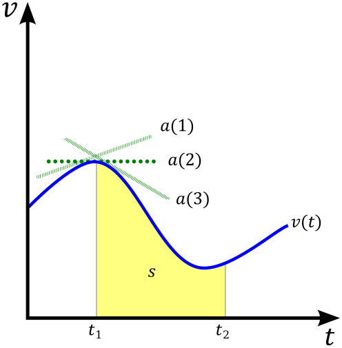
A velocity–time graph for motion with constant acceleration. The straight-line gradient equals acceleration, and the shaded area under the line corresponds to displacement during the time interval. This visual underpins the derivation and use of the SUVAT relationships for uniform acceleration. Source.
These interpretations support the derivation of the SUVAT equations and show their connection to experimental data.
A displacement–time graph provides complementary information: its gradient at any point gives the instantaneous velocity, while changes in the gradient reveal changes in acceleration.
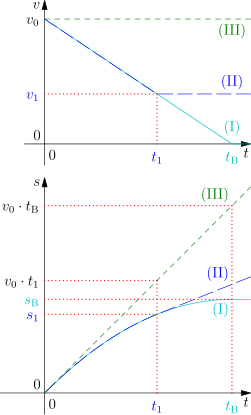
Paired graphs for motion with constant negative acceleration (braking). The speed–time plot has a straight, downward slope (constant deceleration), and the displacement–time curve shows how position evolves during the same interval. This example fits the SUVAT model because the acceleration magnitude is constant. Source.
Application to Free Fall
The acceleration of free fall (g) is approximately 9.81 m s⁻² near the Earth’s surface. In ideal conditions where air resistance is negligible, a freely falling object experiences constant acceleration equal to g.
In such cases, the SUVAT equations apply directly by substituting a = g.
For example:
v = u + gt
s = ut + ½gt²
v² = u² + 2gs
These relationships accurately describe motion during free fall, provided that conditions remain ideal. Real situations, such as air resistance or varying g, require more advanced modelling beyond this specification.
Interpreting Physical Meaning
Each term in the SUVAT equations carries clear physical meaning:
The u t term in displacement represents motion if velocity were constant.
The ½ a t² term accounts for the extra displacement caused by acceleration.
The 2 a s term in the third equation shows how velocity changes are proportional to displacement when acceleration is constant.
Understanding these relationships allows physicists to interpret how motion evolves over time and predict future positions or velocities with precision.
Key Conditions for Using SUVAT Equations
Students must always confirm that:
Acceleration is uniform (no variation with time).
Direction of motion is constant (linear motion).
External forces such as friction or air resistance are negligible, unless specifically included.
When these conditions are not met, alternative mathematical methods such as calculus or numerical analysis must be used.
Practical Use and Measurement
In experimental contexts, determining quantities for use in SUVAT equations involves:
Measuring initial and final velocities using light gates or motion sensors.
Recording time intervals accurately with digital timers.
Calculating acceleration from gradients on velocity–time graphs.
Determining displacement using measured distances or areas under graphs.
Students must link these practical techniques with theoretical equations to validate constant acceleration experimentally.
Summary of Importance
Although each SUVAT equation can be derived from the basic definitions of velocity and acceleration, they remain at the heart of kinematic analysis. Mastery of these relationships enables confident application to free fall, linear motion, and a wide range of mechanical systems within A-Level Physics.
Practice Questions
Question 1 (2 marks)
A car starts from rest and accelerates uniformly at 3.0 m s⁻² for 5.0 s.
Calculate the final velocity of the car after this time.
Mark Scheme:
Substitution into correct SUVAT equation: v = u + at (1 mark)
v = 0 + (3.0 × 5.0) = 15.0 m s⁻¹ (1 mark)
Question 2 (5 marks)
A ball is thrown vertically upwards from the ground with a speed of 12.0 m s⁻¹. Neglect air resistance.
(a) Calculate the maximum height reached by the ball.
(b) Determine the total time taken for the ball to return to the ground.
Mark Scheme:
(a)
Recognition that at maximum height, final velocity v = 0 (1 mark)
Use of v² = u² + 2as with correct substitution: 0 = (12.0)² + 2(−9.81)s (1 mark)
Correct rearrangement and calculation: s = 7.3 m (1 mark)
(b)
Use of v = u + at for upward or downward motion (1 mark)
Example for upward journey: 0 = 12.0 − 9.81t → t = 1.22 sRecognition that total time = 2 × 1.22 = 2.44 s (1 mark)
FAQ
No, the SUVAT equations only apply when acceleration is constant. If acceleration changes with time, the relationships between velocity, displacement, and time are no longer linear or quadratic.
To analyse motion with variable acceleration, physicists use calculus:
Velocity is found by integrating acceleration with respect to time.
Displacement is found by integrating velocity with respect to time.
These methods allow accurate analysis when forces or resistances change during motion.
The ½ arises because acceleration changes velocity linearly over time. The average velocity for uniformly accelerated motion is halfway between the initial and final velocities.
So, displacement = average velocity × time = ((u + v)/2) × t.
Substituting v = u + at gives s = ut + ½at². The ½ term therefore reflects the progressive increase in velocity from u to v under constant acceleration.
Yes. The equations still hold because acceleration due to gravity (g) is constant.
However, the sign convention becomes critical:
Taking upward as positive means g = −9.81 m s⁻² for downward acceleration.
Taking downward as positive means g = +9.81 m s⁻².
The choice of sign direction must be consistent across all terms to ensure accurate results.
They are derived from the definitions of velocity and acceleration:
Acceleration = (change in velocity) / time → a = (v − u) / t → v = u + at.
Average velocity = (u + v) / 2 → displacement = average velocity × time → s = ((u + v)/2)t.
Substituting v = u + at into this gives s = ut + ½at².
Eliminating t from earlier equations gives v² = u² + 2as.
These derivations show that each SUVAT equation is logically consistent with fundamental kinematic definitions.
Experimental setups for motion often rely on timing and distance measurements that can introduce systematic and random errors.
Common issues include:
Timing delays due to human reaction times or sensor lag.
Air resistance reducing effective acceleration below ideal values.
Misalignment of apparatus affecting distance readings.
Using light gates, data loggers, or video analysis improves accuracy by reducing human error and ensuring precise timing, enabling better verification of the SUVAT relationships.
