
OCR Specification focus:
‘Electric current is given by I = A n e v, with n the number density of carriers.’
The continuity equation connects the microscopic motion of charge carriers with the macroscopic current in a conductor, revealing how charge flow depends on material, structure, and properties.
The Continuity Equation in Electrical Conduction
The continuity equation is a fundamental relationship in electricity that links current, charge carrier density, charge, and mean drift velocity. It provides a bridge between microscopic particle behaviour and measurable macroscopic quantities, enabling physicists to understand how materials conduct electric current at the atomic level. This concept is central to analysing current flow in conductors, semiconductors, and other materials where mobile charge carriers are present.
EQUATION
—-----------------------------------------------------------------
Continuity Equation
I = A n e v
I = electric current (ampere, A)
A = cross-sectional area of the conductor (square metre, m²)
n = number density of charge carriers (per cubic metre, m⁻³)
e = elementary charge of a single carrier (coulomb, C)
v = mean drift velocity of carriers (metre per second, m s⁻¹)
—-----------------------------------------------------------------
This equation expresses that the current through a conductor depends on the total number of charge carriers moving through a cross-section each second, multiplied by their individual charge.
Understanding Each Component of the Equation
Electric Current (I)
Electric current represents the rate of flow of electric charge through a conductor. It is measured in amperes (A), where one ampere equals one coulomb of charge passing a point per second. In a wire, this flow arises from the motion of negatively charged electrons or, in electrolytes, from positive and negative ions.
Cross-sectional Area (A)
The cross-sectional area determines how much space is available for charge carriers to move through. A larger area allows more carriers to pass simultaneously, resulting in a greater current for the same drift velocity and carrier density. For instance, a thick copper wire can carry a larger current than a thin one without increasing the speed of the electrons.
Number Density of Charge Carriers (n)
Number Density (n): The number of mobile charge carriers per unit volume of material, typically measured in m⁻³.
The number density is determined by the type of material. Metals have a very high number density because each atom contributes at least one free electron. Semiconductors have much lower values, and insulators possess extremely few mobile charges. This variable directly affects current — if n is small, fewer charge carriers are available to move, so the same current requires a higher drift velocity.
Elementary Charge (e)
Elementary Charge (e): The magnitude of the charge on a single proton or electron, equal to 1.6 × 10⁻¹⁹ coulombs.
Every moving charge contributes a discrete amount of charge to the total current. The concept of quantised charge ensures that current arises from the collective movement of many individual charged particles, each carrying an integer multiple of e. Thus, in metals, the current results from vast numbers of electrons, each with charge −e.
Mean Drift Velocity (v)
The mean drift velocity represents the average velocity of charge carriers due to an applied electric field. Although individual electrons in a metal move randomly and rapidly in all directions, their overall motion superimposes a slow, directed drift towards the positive terminal when a voltage is applied.
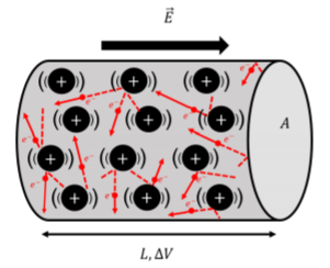
Electron motion inside a conductor is largely random due to frequent collisions, but an applied field produces a small mean drift velocity. The diagram visualises the zig-zag path of a single electron and the net drift direction. This clarifies why vdv_dvd is small even when current is large. Source.
Despite the large current that may flow, drift velocities are typically very small — often less than a millimetre per second — because the number of electrons involved is immense.
Deriving and Interpreting the Equation
The relationship I = A n e v can be understood by considering the rate at which charge passes through a cross-section of the conductor:
Each carrier has charge e.
In a volume of A × v × 1 s, all carriers move a distance v in one second.
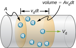
Schematic of a conductor segment of cross-sectional area AAA whose carriers drift a distance vd dtv_d\,dtvddt in time dtdtdt. The shaded volume contains nAvddtnA v_d dtnAvddt carriers, each of charge qqq, giving I=qnAvdI = q n A v_dI=qnAvd. This directly illustrates the continuity equation linking microscopic motion to macroscopic current. Source.
The total number of carriers in this volume is n × A × v.
The total charge that passes the section each second is therefore Q = n e A v.
Since current I = Q/t, and the time considered is one second, the equation follows directly.
This derivation shows that current depends not on how fast individual electrons move at random, but on their average drift velocity multiplied by their number density and the available area for flow.
Applications and Implications
Relationship Between Material and Current Flow
Metals: High number density (n), allowing large current even with small drift velocities.
Semiconductors: Intermediate n, so drift velocity must increase to maintain current.
Insulators: Negligible n, meaning almost no current flows under normal conditions.
Thus, the continuity equation underpins why different materials conduct electricity to varying degrees and explains the microscopic basis for Ohm’s law and other macroscopic relationships.
Effects of Conductor Dimensions
When the cross-sectional area A is increased, more charge carriers can move simultaneously, reducing the current density (current per unit area). This is essential for designing safe electrical systems — larger wires prevent overheating by keeping drift velocity and resistive heating low for a given current.
Influence of Electric Field and Potential Difference
An applied potential difference produces an electric field that accelerates charge carriers. As a result, drift velocity v increases, and hence current I increases proportionally, assuming A, n, and e remain constant. This explains the direct relationship between potential difference and current in ohmic materials where resistance is constant.
Quantitative and Qualitative Insights
Although the equation looks simple, it captures a profound physical relationship:
It reveals how microscopic motion of charges translates into measurable current.
It clarifies why even a slow drift of electrons can produce a substantial current due to the immense number of carriers.
It demonstrates how changes in material type or geometry alter electrical behaviour.
In essence, the continuity equation provides the fundamental connection between the atomic world of moving charges and the observable electrical quantities central to circuit theory.
Practice Questions
Question 1 (2 marks)
State the equation linking current I, cross-sectional area A, number density of charge carriers n, charge of each carrier e, and mean drift velocity v.
Explain briefly what is meant by mean drift velocity.
Mark scheme
1 mark: Correct equation stated: I = A n e v
1 mark: Mean drift velocity described as the average velocity of charge carriers along a conductor due to an applied electric field (not random motion).
Question 2 (5 marks)
A copper wire of circular cross-section has a diameter of 1.2 mm and carries a current of 2.0 A. The number density of free electrons in copper is 8.5 × 10²⁸ m⁻³ and the charge of an electron is 1.6 × 10⁻¹⁹ C.
(a) Calculate the mean drift velocity of electrons in the wire. (4 marks)
(b) Explain why, despite the large current, the drift velocity is very small. (1 mark)
Mark scheme
(a)
1 mark: Recognises use of I = A n e v.
1 mark: Calculates cross-sectional area A = πr² = π(0.6 × 10⁻³)² = 1.13 × 10⁻⁶ m².
1 mark: Substitutes correctly into v = I / (A n e).
v = 2.0 / (1.13 × 10⁻⁶ × 8.5 × 10²⁸ × 1.6 × 10⁻¹⁹).1 mark: Correct numerical result with suitable units: v ≈ 1.3 × 10⁻⁴ m s⁻¹.
(b)
1 mark: Explanation — although individual electrons move rapidly in random directions, their net drift due to the applied field is small because of the very high number density of electrons.
FAQ
The derivation assumes a steady current, meaning that charge does not accumulate anywhere in the conductor. It also assumes a uniform cross-sectional area and a constant number density of charge carriers throughout the material.
The drift velocity is taken as the same for all carriers, and the flow is considered to be linear and continuous. These assumptions allow the relationship between microscopic motion and macroscopic current to remain valid for metals and steady-state conditions.
As temperature increases, metal ions vibrate more vigorously, leading to more frequent collisions between electrons and ions. This increases electrical resistance.
For a given potential difference, the current decreases slightly, so the mean drift velocity also decreases. However, if the current is maintained constant by an external source, a higher electric field is required to compensate for the increased resistance.
It is called the continuity equation because it expresses the continuous flow of electric charge through a conductor. The total charge passing through any cross-section per second remains constant in a steady current.
This continuity reflects the conservation of charge, implying that charge cannot be created or destroyed within the conductor — it can only move from one region to another.
In DC circuits, the drift velocity has a constant direction and magnitude over time, corresponding to steady charge flow.
In AC circuits, the direction of the electric field — and therefore the drift velocity — reverses periodically, typically 50 times per second in the UK. Although the average drift velocity over time is zero, energy transfer still occurs as electrons oscillate back and forth, transferring energy to the circuit components.
Yes, but with caution.
In semiconductors, both electrons and holes act as charge carriers, each with their own number density and charge. The total current is the sum of the contributions from both types of carrier.
In electrolytes, positive and negative ions move in opposite directions, each contributing to the overall current according to their charge and drift velocity.
The principle remains the same — current equals the rate of charge flow — but multiple carrier types must be considered.
