Approximating definite integrals is essential when an exact antiderivative is unknown. By using information from graphs, tables, formulas, or descriptions, students estimate accumulated change accurately.

Approximating Integrals from Graphs and Tables

When a function cannot be integrated exactly or a closed-form antiderivative is unavailable, numerical approximation provides a practical method for estimating a definite integral, which represents accumulated change over an interval. This subsubtopic focuses on constructing approximations when the function is presented visually, numerically, algebraically, or contextually. The goal is to interpret available information to approximate the area under a curve with justified methods.

Understanding the Goal of Numerical Approximation

A definite integral such as $\int_a^b f(x),dx$ measures the accumulated change of a quantity over the interval $[a,b]$. When the explicit antiderivative is not accessible or when data is incomplete, numerical methods approximate this accumulation. These estimates rely on constructing geometric regions whose areas mimic the behavior of the function over small subintervals.

Key Situations Requiring Approximation

Students must recognize the diverse contexts in which approximation becomes necessary. These contexts determine how the integral will be estimated and influence which numerical strategy is most appropriate.

• Graph-only information
  When the graph of $f(x)$, but not its equation, is provided, estimation depends on visual interpretation. Students rely on reading heights at specific points, observing curvature, and segmenting the domain into usable subintervals.

• Tabular data
  When values of $f(x)$ are listed for discrete $x$-values, the function’s behavior between recorded points is unknown. Numerical methods approximate the area by assuming reasonable behavior between these known values.

• Analytical expressions
  When a function is given explicitly and is difficult or impossible to integrate symbolically at the AP level, its values can be computed at selected points and used in numerical approximations.

• Verbal descriptions
  When a function is given in words, important quantitative details—such as constant rates, linear trends, or periodic behavior—must be extracted and interpreted numerically.

Interpreting Graphs for Approximation

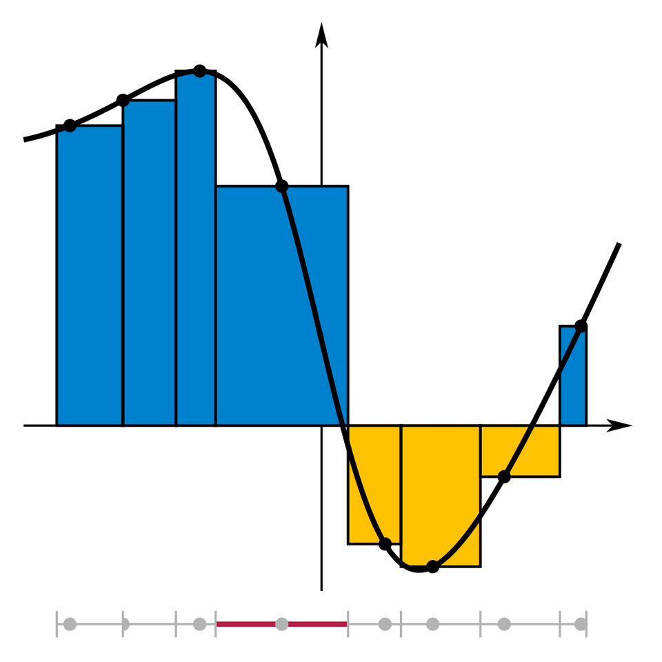
To approximate the area under $y=f(x)$ from a graph, we divide $[a,b]$ into subintervals and draw rectangles whose heights come from function values at chosen $x$-coordinates.

Graph of a function with a Riemann sum approximation using vertical rectangles. Each rectangle’s height equals the function value at a selected point in its subinterval, while the width is the subinterval length. One interval is highlighted to show how different widths and sample positions affect the approximation. Source.

Important considerations include:

• Identifying equally spaced or unevenly spaced $x$-values along the interval.

• Estimating the function’s height at endpoints, midpoints, or other sample points.

• Recognizing whether the function is increasing or decreasing, which affects overestimates and underestimates.

• Evaluating regions where the function crosses the x-axis, noting that areas below the axis contribute negative accumulated change.

Interpreting Tables for Approximation

When working with tables, students must pay careful attention to the spacing of $x$-values and to the behavior implied by discrete measurements.

Key steps include:

• Determining subinterval widths, which may be uniform or nonuniform.

• Identifying which provided function values correspond to left endpoints, right endpoints, or midpoints.

• Ensuring consistent pairing of widths and heights in the approximation method chosen.

• Accounting for sign changes when the table indicates negative values of $f(x)$.

Numerical Methods in Context

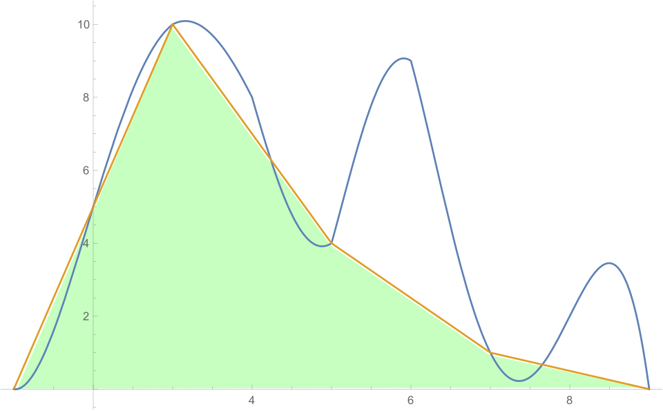
Another common numerical method uses straight-line segments between consecutive points on the graph so that each curved strip is approximated by a trapezoid instead of a rectangle.

Trapezoidal approximation of the area under a curve using four subintervals. Straight-line segments connect consecutive function values to form trapezoids whose areas approximate the integral. This image includes a specific numerical method, the trapezoidal rule, which fits within the broader topic of estimating integrals from graphical information. Source.

Common triggers for selecting an approximation method include:

• The presence of discrete data naturally leading to endpoint or midpoint approximations.

• Graphs with clearly linear behavior on subintervals suggesting trapezoidal estimates.

• Situations where the function value is easiest to read or infer at specific points.

Essential Interpretive Skills

Accurate approximation requires interpreting the meaning and implications of the available information. Students must develop the following competencies:

• Distinguishing visual trends, such as concavity or linearity, that influence how well simple geometric regions approximate the actual area.

• Connecting numerical values to geometric reasoning, ensuring that function values correspond correctly to heights of rectangles or trapezoids.

• Assessing reasonableness by considering whether an approximation seems too large or too small based on the graph or table.

• Using contextual cues from word-based descriptions, such as constant or varying rates, to guide the selection of subintervals and sampling points.

Communicating Approximation Results

In AP Calculus AB, students must clearly explain their reasoning when presenting an approximation. This includes identifying:

• The interval of approximation.

• The points at which the function is sampled.

• The widths used in constructing subintervals.

• The method employed and its justification based on available information.

Approximations as Tools for Understanding Accumulated Change

When function values are available only at several points on a graph or in a table, we can think of each value as the height of a rectangle over its subinterval and add those areas to approximate the integral.

Graph of a nonnegative function on $[0,1]$ with vertical rectangles approximating the area under the curve. Each rectangle corresponds to a subinterval and uses the function value at an endpoint as its height. The source page also discusses limits and exact definite integrals, which extend beyond the visual approximation highlighted here. Source.

Numerical approximation deepens conceptual understanding by emphasizing that definite integrals represent accumulation, even when the precise antiderivative cannot be found. Approximating from graphs, tables, formulas, or descriptions reinforces the idea that integration is fundamentally connected to area and that accumulated change can be estimated reliably with limited information.