
AP Syllabus focus: ‘The output gap is the difference between actual output and potential output.’
The output gap is a core way to describe where the economy is in the business cycle.
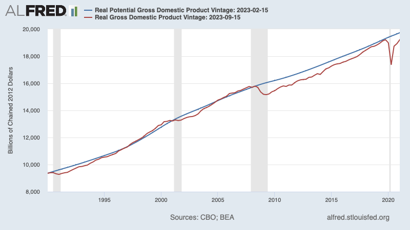
Actual real GDP and potential real GDP are plotted together over time, so the vertical distance between the two lines represents the output gap in level terms. When the actual GDP line falls below potential GDP, the economy is operating with slack (a recessionary gap); when it rises above, the economy is overheating (an inflationary gap). Source
It compares actual real GDP to the economy’s sustainable level of production, helping predict unemployment pressures and inflationary risks.
What the output gap measures
Output gap: The difference between actual real GDP and potential real GDP at a point in time.
A gap exists because short-run spending and production can deviate from what the economy can produce when labour and capital are fully and efficiently employed.
Actual vs potential output
Potential output (potential real GDP): The level of real GDP the economy can produce when operating at full employment, given current technology, resources, and institutions.
Potential output is not the maximum physically possible output; it is the sustainable level consistent with normal frictions in labour markets and typical capacity use.
Calculating and expressing the output gap
The output gap is most often stated in real (inflation-adjusted) terms and can be expressed either as a dollar (level) difference or as a percentage of potential output.
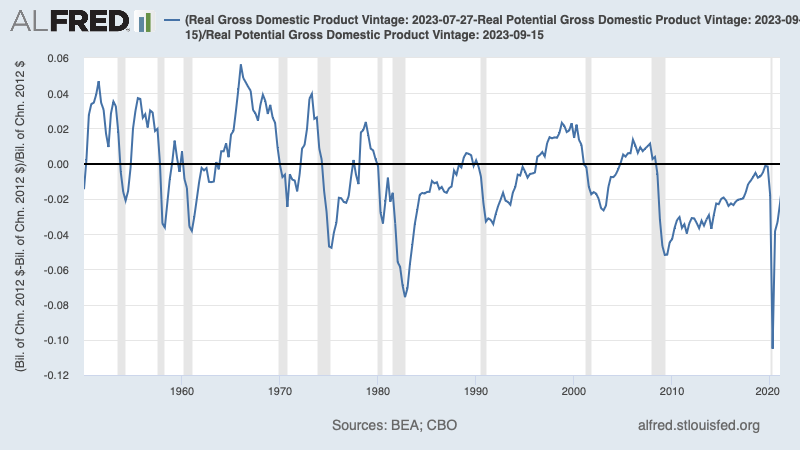
The output gap is shown as a time series measured in percent of potential GDP, with the zero line marking . Values below zero indicate a negative (recessionary) gap, while values above zero indicate a positive (inflationary) gap. Shaded recession bands help connect persistent negative gaps to downturns in the business cycle.Source
= actual real GDP, in dollars
= potential real GDP, in dollars
= gap as a percentage of potential GDP, in percent
A positive value indicates the economy is producing above potential; a negative value indicates production below potential.
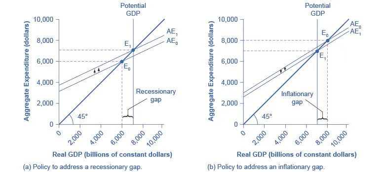
Two Keynesian-cross panels show how equilibrium output can fall short of potential GDP (recessionary gap) or exceed it (inflationary gap). The bracketed horizontal distance between equilibrium real GDP and the vertical potential GDP line is the gap. The diagram also illustrates the policy intuition: shifting aggregate expenditure can move equilibrium back toward potential output. Source
Interpreting the sign: recessionary vs inflationary gaps
Negative output gap (recessionary gap)
When , the economy has a recessionary gap:
Idle resources: firms operate below normal capacity; layoffs and reduced hours are more likely.
Unemployment pressure: cyclical unemployment tends to rise as output falls short of potential.
Inflation pressure: downward pressure on inflation can occur because weak demand reduces firms’ pricing power.
Positive output gap (inflationary gap)
When , the economy has an inflationary gap:
Resource strain: labour markets tighten; overtime and capacity constraints become common.
Rising costs: wages and input prices may accelerate as firms compete for scarce resources.
Inflation pressure: sustained demand above potential tends to increase inflation.
Why the output gap matters for macroeconomic goals
Policymakers care about the output gap because it connects directly to two key outcomes:
Stabilisation: closing a recessionary gap supports higher employment and output.
Price stability: reducing an inflationary gap helps limit demand-pull inflation.
The output gap is therefore a practical summary of whether aggregate spending is too low or too high relative to the economy’s productive capacity, even when real GDP is still growing.
Measurement challenges (what students should remember)
The output gap depends on estimating potential output, which cannot be observed directly. As a result:
potential output estimates can change as new data arrive or methods are updated,
productivity shifts or changes in labour force trends can move ,
the output gap can be revised significantly after initial publication, complicating real-time policy decisions.
Practice Questions
(2 marks) Define the output gap and state what it means when the output gap is negative.
1 mark: Correct definition: difference between actual output (real GDP) and potential output.
1 mark: Negative gap means actual real GDP is below potential (recessionary gap / underutilised resources).
(6 marks) Using the concept of the output gap, explain how an economy can experience inflationary pressure even when real GDP is increasing.
1 mark: Identifies that the output gap compares to (potential output).
1 mark: Explains that real GDP can be increasing while exceeds (positive output gap).
1 mark: Links positive output gap to resource constraints/tight labour markets/capacity limits.
1 mark: Explains rising wages/input costs when resources are scarce.
1 mark: Connects cost increases and/or excess demand to upward pressure on the price level (inflation).
1 mark: States that sustained production above potential is associated with demand-pull inflation risk.
FAQ
They use statistical filters, production-function approaches, and estimates of trend productivity and trend labour input.
Different methods can produce different $Y^*$ paths, especially around turning points.
Revisions occur when:
real GDP data are revised,
trend growth assumptions change,
structural changes (productivity, participation) are reassessed.
Revisions can alter the perceived sign and size of the gap in past years.
Yes, if potential output changes. For example, slower productivity growth or reduced labour force growth can lower $Y^*$, shrinking a negative gap even if $Y$ is flat.
Conversely, faster trend growth can widen a gap without a fall in $Y$.
It suggests sustained demand above capacity, which can:
encourage short-run overutilisation of labour and capital,
increase wage and price pressures,
raise the likelihood that inflation becomes embedded in expectations.
They are conceptually similar: both capture how intensively resources are used.
Capacity utilisation is often sector-specific and based on surveys; the output gap is economy-wide and model-based, so the two can diverge when some sectors are constrained and others are slack.
