Instantaneous kinematics uses the limiting behavior of average motion over very small time intervals. Calculus then connects motion functions, allowing precise relationships among position, velocity, and acceleration at any moment.

The Limiting Idea

In kinematics, a function such as $x(t)$ gives the position of an object at each time $t$. The value of $x(t)$ at one specific instant is the object’s instantaneous position. Unlike an average quantity, it does not describe a whole interval; it describes a single moment.

Average quantities are often easier to measure first, but they do not capture exactly what is happening at one instant. The key AP Physics C idea is that an instantaneous value is found by shrinking the time interval until it becomes arbitrarily small. This is the limiting process that leads to derivatives.

A central quantity is instantaneous velocity.

Average velocity over a finite interval uses the ratio of change in position to change in time. Taking the limit of that ratio gives the derivative of position with respect to time.

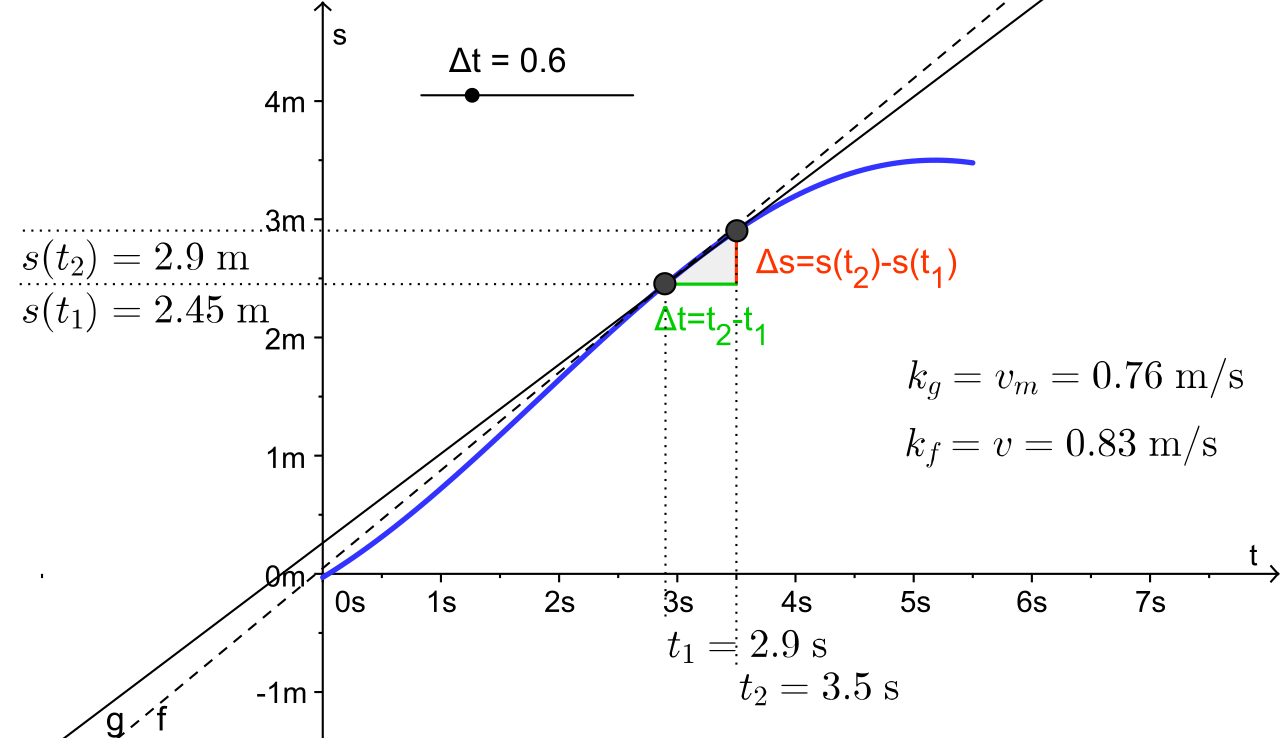
On a position–time graph, the average velocity over a finite interval corresponds to the slope of a secant line, while the instantaneous velocity at a moment corresponds to the slope of the tangent line. As the interval shrinks ($\Delta t\to 0$), the secant slope approaches the tangent slope, illustrating $v(t)=dx/dt$ geometrically. Source

This derivative tells how rapidly position is changing at that exact instant. A positive value means the coordinate is increasing at that moment, while a negative value means it is decreasing.

Another essential quantity is instantaneous acceleration.

Just as velocity comes from how position changes, acceleration comes from how velocity changes. It is the derivative of velocity with respect to time.

The final form, $a(t)=d^2x/dt^2$, shows that acceleration is the second derivative of position. If position is known as a function of time, velocity and acceleration follow from differentiation.

Differentiation Connects the Motion Functions

Differentiation is the mathematical operation that turns one motion function into the next. In one-dimensional motion:

• $x(t)$ describes where the object is

• $v(t)=dx/dt$ describes how quickly position is changing

• $a(t)=dv/dt$ describes how quickly velocity is changing

These are not separate ideas.

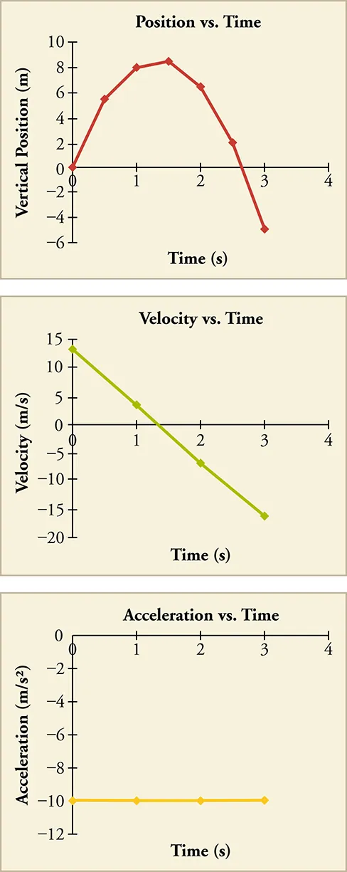
A matched set of $x(t)$, $v(t)$, and $a(t)$ graphs for the same motion highlights how differentiation and integration connect kinematic quantities. The slope of $x(t)$ at each time gives $v(t)$, and the slope of $v(t)$ gives $a(t)$; with constant acceleration, $a(t)$ is a horizontal line while $v(t)$ is linear and $x(t)$ is curved (quadratic). Source

They are linked descriptions of the same motion. Because of this connection, knowing one function can allow you to determine another, provided the function is expressed in terms of time and is differentiable.

The derivative is local, meaning it depends on behavior very near the chosen time. That is why an object can have different instantaneous velocities at nearby times even if its overall trip seems simple. Instantaneous quantities describe motion with much more detail than averages do.

Integration Reverses the Process

Integration reverses differentiation. If acceleration is known as a function of time, integration gives the change in velocity over a time interval. If velocity is known, integration gives the change in position.

These integrals give changes over an interval, not automatically the final values themselves. To identify a unique motion, you must combine the integral result with the object’s value at some starting time. For example, final velocity is found from $v_f=v_i+\Delta v$, and final position is found from $x_f=x_i+\Delta x$.

This is why AP Physics C often treats motion as a chain of related functions rather than isolated formulas. Differentiation moves from position to velocity to acceleration. Integration moves back from acceleration to velocity and from velocity to position.

Physical Meaning at an Instant

Instantaneous quantities should be interpreted carefully.

Instantaneous Position

The position $x(t)$ tells the object’s coordinate at one exact time. It does not say how the object got there or how it will move next. Two different motions can pass through the same position at the same instant.

Instantaneous Velocity

Velocity describes motion at that moment, not over a long interval.

• If $v(t)>0$, the position coordinate is increasing

• If $v(t)<0$, the position coordinate is decreasing

• If $v(t)=0$, the object is momentarily at rest in that coordinate system

A zero instantaneous velocity does not, by itself, determine the acceleration.

Instantaneous Acceleration

Acceleration describes how the velocity is changing at that moment.

• If $a(t)>0$, velocity is changing in the positive direction

• If $a(t)<0$, velocity is changing in the negative direction

• If $a(t)=0$, velocity is not changing at that instant

Acceleration is tied directly to velocity, not directly to position.

Common Checks and Pitfalls

When working with instantaneous motion, keep these ideas in mind:

• Limits matter: an instantaneous quantity comes from a limiting process, not from choosing a merely small time interval

• Units matter: differentiating position gives meters per second, and differentiating velocity gives meters per second squared

• Integration gives change: you still need starting information to recover the full motion

• A derivative may fail to exist at a time where a motion function has a sharp corner, cusp, or jump