The Empirical Rule gives quick approximate percentages for data in an approximately normal setting, linking the center and spread of a distribution to familiar benchmarks used often in AP Statistics.

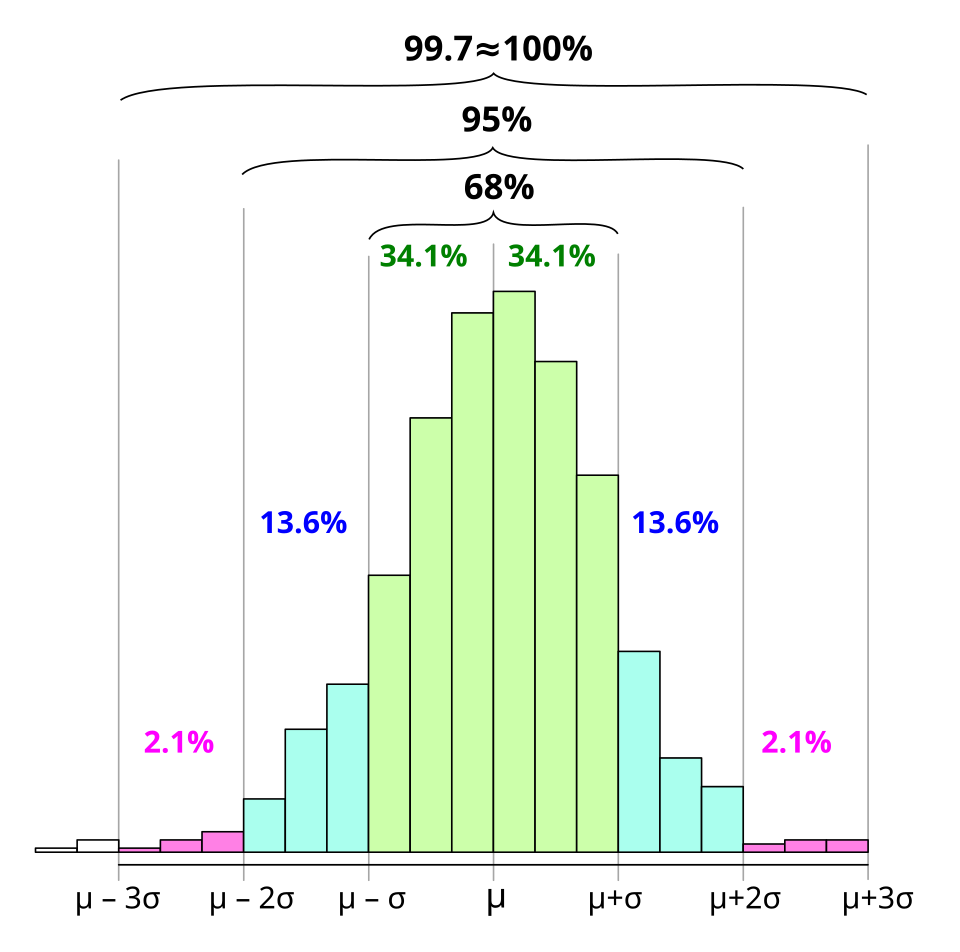
A histogram illustrating the Empirical Rule regions around the mean, with the central mass partitioned by standard-deviation cut points. This helps students connect the theoretical 68–95–99.7 benchmarks to the appearance of approximately normal data in a plot. Source

The core idea

In a normal distribution, observations cluster near the mean and become less common as you move away from the center. The Empirical Rule turns that visual pattern into three benchmark percentages that are easy to remember and apply.

This rule depends on two ideas. The mean gives the center of the distribution, and the standard deviation measures how far observations typically vary from that center. The relevant intervals are from $\mu-\sigma$ to $\mu+\sigma$, from $\mu-2\sigma$ to $\mu+2\sigma$, and from $\mu-3\sigma$ to $\mu+3\sigma$.

The three benchmark percentages

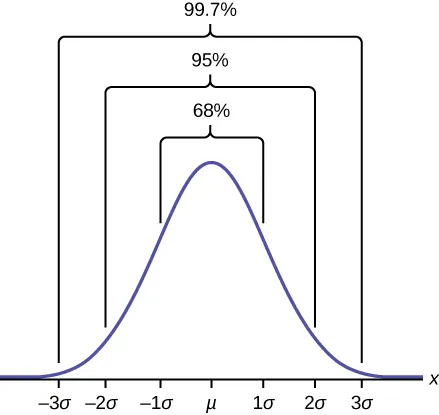
A normal (bell-shaped) curve with brackets marking the central 68%, 95%, and 99.7% regions. The x-axis is labeled in standard-deviation units from $-3\sigma$ to $3\sigma$ around the mean $\mu$, making the nested nature of the three intervals visually explicit. Source

• About 68% of observations are within 1 standard deviation of the mean.

• About 95% of observations are within 2 standard deviations of the mean.

• About 99.7% of observations are within 3 standard deviations of the mean.

Because a normal distribution is symmetric, these percentages are split evenly on the left and right sides of the mean.

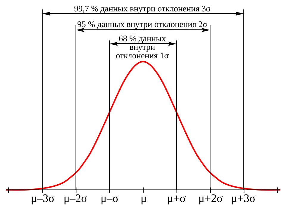
A normal-curve diagram marking standard-deviation positions from $-3\sigma$ to $3\sigma$ and the cumulative Empirical Rule coverage. It visually supports splitting probabilities into symmetric left and right tails, which is the key idea behind “each tail” percentages. Source

• If about 68% are within 1 standard deviation, then about 32% are outside that interval, or about 16% in each tail.

• If about 95% are within 2 standard deviations, then about 5% are outside that interval, or about 2.5% in each tail.

• If about 99.7% are within 3 standard deviations, then about 0.3% are outside that interval, or about 0.15% in each tail.

How to interpret the rule

The phrase within 1 standard deviation means all observations from one standard deviation below the mean to one standard deviation above the mean. The same structure applies for 2 and 3 standard deviations.

These percentages describe the proportion of observations expected in those intervals when the distribution is normal. They are not guarantees about every single sample. Instead, they are reliable approximations for a distribution that follows the normal model well.

For AP Statistics, interpretation in context matters. A correct statement should connect the percentage to the interval around the mean.

• About 68% means a little more than two-thirds of observations are fairly close to the center.

• About 95% means almost all observations are within a moderate distance of the center.

• About 99.7% means nearly every observation is within a fairly wide interval centered at the mean.

The rule is especially useful for identifying how unusual an observation might be. In a normal distribution:

• A value more than 2 standard deviations from the mean is relatively uncommon.

• A value more than 3 standard deviations from the mean is very unusual.

Why the rule matters

The Empirical Rule is important because it gives quick approximate answers without lengthy calculations or technology. It connects a distribution’s shape, center, and spread in one compact idea.

It helps you:

• estimate the proportion of observations in an interval centered at the mean

• judge whether an observed percentage seems reasonable for normal data

• connect the standard deviation to the overall spread of the distribution

• recognize whether a value is common, uncommon, or very unusual

It also gives a mental picture of how observations are distributed. Most values lie near the middle, fewer appear farther away, and only a tiny fraction appear in the extreme tails. That pattern is exactly what the normal model represents.

When you should use it

Use the Empirical Rule only when the distribution is normal or approximately normal. It is not a shortcut for every quantitative data set.

If a distribution departs clearly from normality, the 68-95-99.7 pattern may not describe the data well. In that case, using the rule can lead to misleading interpretations.

The word about is essential. Even for a population that is exactly normal, the familiar percentages are rounded. For actual data, observed percentages will usually be close to these values rather than exact matches.

When interpreting the rule, be specific. A complete statement should include both:

• the interval, described by how many standard deviations from the mean

• the approximate percentage of observations in that interval

Saying only that observations are “close to the mean” is too vague. The Empirical Rule is valuable because it gives a more precise description of what “close” means in a normal setting.

Common interpretation issues

• The 95% within 2 standard deviations includes the 68% within 1 standard deviation. These are nested intervals, not separate groups.

• The rule describes overall proportions in a normal distribution, not certainty about any individual observation.

• The rule does not say observations beyond 2 or 3 standard deviations are impossible. It says they are uncommon or very rare.

• The intervals are always centered at the mean, not at some other point on the scale.

• A data set is not proved normal just because some percentages look close to 68%, 95%, and 99.7%. The Empirical Rule describes normal distributions; it does not by itself establish that one is present.