Normal distributions let us connect areas under a curve to proportions and cutoff values. In AP Statistics, you should be able to move from values to areas and from areas back to values using tables or technology.

Areas Under a Normal Curve

In a normal model, the total area under the curve is 1, so any area represents a proportion of observations.

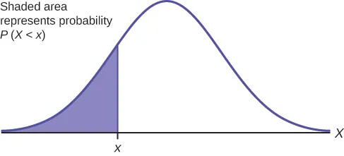
A normal density curve with the region to the left of a cutoff value $x$ shaded. The shaded area is labeled as the probability $P(X<x)$, illustrating the interpretation of cumulative (left-tail) area as a proportion of observations. Source

The same area can also be interpreted as a probability for a randomly selected observation from that model. When a question asks for the proportion less than a value, greater than a value, or between two values, it is asking for an area under the normal curve.

• A left-tail area gives the proportion below a boundary.

• A right-tail area gives the proportion above a boundary.

• An area between two values gives the proportion in that interval.

A percentile identifies a location in the distribution rather than an area itself.

Percentiles reverse the usual question. Instead of starting with a data value and finding an area, you start with an area or percentage and find the value that cuts off that proportion. For instance, the 90th percentile is the value with 90% of observations at or below it.

Standardizing and Using Tables

Standard normal tables are built for the standard normal distribution, which has mean 0 and standard deviation 1. If a variable has some other normal mean and standard deviation, convert the original value to a standardized value before using the table.

After standardizing, locate the row and column for the $z$-value.

Most AP Statistics tables give the cumulative area to the left of $z$, written as $P(Z\le z)$. Some tables use a different convention, such as area between the mean and $z$, so always read the heading before interpreting a value.

When a problem involves an interval, combine table areas carefully.

• For a value less than a boundary, use the left cumulative area.

• For a value greater than a boundary, subtract the left area from 1.

• For a value between two boundaries, find both cumulative areas and subtract the smaller from the larger.

• For a value outside an interval, either add the two tail areas or subtract the middle area from 1.

Tables are especially useful for showing the connection between standardized values and areas, but they usually require rounding the $z$-score to two decimal places. That means table answers are approximations, not exact values.

Using Technology and Computer Output

Technology often works directly with the original normal model, so it reduces both setup time and rounding error. Graphing calculators, statistical software, and online tools can compute normal areas and inverse normal cutoffs without needing a separate table lookup.

Finding Proportions on Intervals

To find a proportion with technology, enter the lower bound, upper bound, mean, and standard deviation. The output is the area under the normal curve between those bounds.

• For a left-tail proportion, use a very small lower bound or a negative infinity option if available.

• For a right-tail proportion, use a very large upper bound, an infinity option, or subtract a left-tail area from 1.

• For a middle proportion, use both endpoints directly.

Computer output may display a decimal such as 0.842 or a percentage such as 84.2%. These represent the same proportion. Report the result in the form requested by the question, and include context when interpreting it.

Estimating Values from Areas

If you are given a percentile or an area and asked for the corresponding data value, use an inverse normal calculation.

A graph depicting the inverse of the normal distribution, emphasizing the idea of going from probability (area) back to a corresponding cutoff value (a quantile). This supports the conceptual goal of inverse normal calculations: translating a target cumulative proportion into a boundary on the measurement scale. Source

This finds the cutoff value whose left-tail area matches the requested proportion.

• Convert a percentile to a cumulative proportion.

• Use the target area together with the mean and standard deviation.

• If the question gives an upper-tail proportion, rewrite it as a left-tail area before using inverse normal.

• State the answer in original units, not as a $z$-score, unless the question specifically asks for the standardized value.

This idea is important because AP Statistics questions often move in both directions: from a score to a proportion, and from a proportion to a score.

Interpreting Results Correctly

When you read an area from a table or technology output, be clear about what it means. An area does not describe the height of the curve. It describes the share of observations in a region of the distribution.

• A proportion of 0.25 means about 25% of observations are in that region.

• A percentile is a cutoff value, not the percentage itself.

• A result found from a normal model is an estimate based on that model.

• Units matter: proportions have no units, but percentile cutoffs use the original measurement units.

A quick reasonableness check can prevent mistakes. Values far above the mean should have large left-tail areas and small right-tail areas. Values near the mean should have left-tail areas near 0.50. Symmetry also helps: equal distances on opposite sides of the mean have matching tail areas.

In AP responses, accuracy and interpretation both matter. Use the correct area, keep track of whether the question is asking for a proportion or a cutoff value, and express the final answer in the language of the context.