
AQA Specification focus:
‘How to use AD/AS diagrams to illustrate macroeconomic equilibrium.’
Understanding how aggregate demand (AD) and aggregate supply (AS) interact is central to macroeconomics, as their intersection defines macroeconomic equilibrium, showing output and the overall price level.
Understanding Macroeconomic Equilibrium
Macroeconomic equilibrium occurs where the aggregate demand (AD) curve intersects the aggregate supply (AS) curve. At this point, planned spending in the economy matches planned production, meaning there are no unintended changes in inventories.
Macroeconomic Equilibrium: The state where aggregate demand equals aggregate supply, determining the equilibrium price level and real national output.
At equilibrium, the economy produces a level of real GDP consistent with the price level, reflecting the balance between the total demand for goods and services and the total supply.
The Aggregate Demand Curve and Movements
The AD curve shows the relationship between the price level and total demand for real output. Movements along the AD curve result from changes in the general price level, not from shifts in its determinants.
A fall in the price level → movement along AD showing higher real output demanded.
A rise in the price level → movement along AD showing lower real output demanded.
The Aggregate Supply Curve and Its Variants
The AS curve represents the relationship between the price level and the total quantity of goods and services supplied. It has two important forms:
Short-run aggregate supply (SRAS): Upward sloping, reflecting that higher prices may encourage firms to increase production.
Long-run aggregate supply (LRAS): Vertical, showing the economy’s productive capacity determined by resources, technology, and institutions.
Short-Run Aggregate Supply (SRAS): The total planned output of goods and services at different price levels when some costs are fixed.
This distinction is crucial for showing how equilibrium changes in both the short run and the long run.
Equilibrium in AD/AS Diagrams
In AD/AS diagrams, equilibrium is shown at the intersection point of AD and AS:
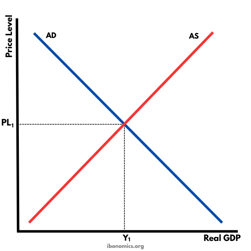
This diagram depicts the short-run macroeconomic equilibrium where the AD and SRAS curves intersect, determining the equilibrium price level and real GDP. The diagram is simplified to focus on the equilibrium point, aligning with the AQA A-Level Economics syllabus. Source
The x-axis represents real GDP (national output).
The y-axis represents the general price level.
The equilibrium point shows the simultaneous determination of real GDP and the price level.
When the AD curve intersects the SRAS curve, the economy is in short-run equilibrium. If the intersection also lies on LRAS, the economy is in long-run equilibrium at full capacity.
Disequilibrium Situations
If the economy is not at the AD-AS intersection, disequilibrium occurs:
Excess demand: AD exceeds AS at the current price level, creating inflationary pressure.
Excess supply: AS exceeds AD at the current price level, creating downward pressure on prices and possible unemployment.
Excess Demand: A situation where aggregate demand exceeds aggregate supply at the prevailing price level, leading to upward pressure on prices.
Shifts in Equilibrium
Equilibrium changes when either AD or AS shifts. These shifts alter the intersection point, creating a new equilibrium.
Shifts in Aggregate Demand
Factors such as changes in consumption, investment, government spending, or net exports can shift AD. For example:
An increase in government spending shifts AD rightwards, raising both equilibrium output and the price level.
A fall in consumer confidence shifts AD leftwards, reducing equilibrium output and price levels.
Shifts in Aggregate Supply
Cost changes, productivity improvements, or changes in resource availability can shift SRAS or LRAS:
A rise in wage costs shifts SRAS leftwards, causing lower output and higher prices.
Technological advances shift LRAS rightwards, raising the economy’s capacity and long-term output.
Interaction of Short-Run and Long-Run Equilibrium
In the short run, equilibrium may be at a level below or above full employment output. However, in the long run, the economy tends towards an equilibrium at LRAS:
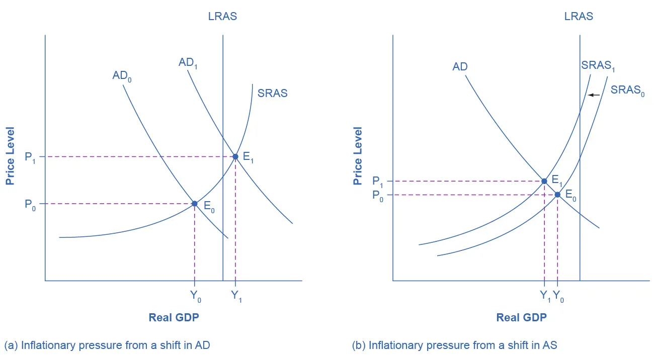
This diagram illustrates the long-run macroeconomic equilibrium where the AD, SRAS, and LRAS curves intersect at the economy's potential output. It highlights the concept of full employment and the natural rate of output, as per the AQA A-Level Economics specification. Source
If AD intersects SRAS to the left of LRAS → recessionary gap.
If AD intersects SRAS to the right of LRAS → inflationary gap.
When AD, SRAS, and LRAS all meet → long-run full employment equilibrium.
National Income Identity (Y) = C + I + G + (X – M)
C = Consumption
I = Investment
G = Government spending
X = Exports
M = Imports
This equation underpins the components of AD, which in turn determine the equilibrium with AS.
Visualising Equilibrium with AD/AS Diagrams
In practice, students must use AD/AS diagrams to illustrate equilibrium changes:
Start with initial equilibrium at AD and SRAS intersection.
Show the effect of shifts by drawing new curves and identifying the new intersection point.
Use LRAS to highlight whether the economy is at full capacity.
Importance of AD/AS Equilibrium Analysis
Using AD/AS to show equilibrium allows economists to:
Analyse inflation, unemployment, and growth.
Understand how policy changes (fiscal or monetary) affect output and prices.
Connect global events, such as oil price shocks, to domestic equilibrium outcomes.
By mastering AD/AS equilibrium analysis, students can apply diagrams directly to macroeconomic problems, fulfilling the AQA specification requirement.
Practice Questions
Using an aggregate demand and aggregate supply diagram, identify the equilibrium price level and level of real output. (2 marks)
1 mark for correctly identifying the equilibrium price level where AD and AS intersect.
1 mark for correctly identifying the equilibrium level of real output where AD and AS intersect.
Explain, using an aggregate demand and aggregate supply diagram, how an increase in government spending can affect macroeconomic equilibrium in both the short run and the long run. (6 marks)
Up to 2 marks for a clear diagram showing a rightward shift of the AD curve.
1 mark for identifying that in the short run, the new equilibrium shows higher real output and a higher price level.
1 mark for identifying that in the long run, if the economy is at full capacity, the increase in AD leads mainly to inflationary pressure rather than sustained output growth.
1 mark for clear explanation of the difference between short-run and long-run effects.
1 mark for correct use of key terms such as “inflationary gap”, “full employment output”, or “long-run aggregate supply”.
FAQ
Short-run equilibrium occurs when AD intersects SRAS, which can be at any level of output depending on demand conditions. This might be below, at, or above full employment.
Long-run equilibrium is only achieved when AD, SRAS, and LRAS all meet at the full employment level of output. Here, the economy is producing at its potential capacity without inflationary or recessionary gaps.
Equilibrium output may not always align with full employment output because AD can intersect SRAS at a point away from LRAS.
If output is below LRAS, a negative output gap exists, signalling unemployment.
If output is above LRAS, a positive output gap occurs, creating inflationary pressure.
These gaps reflect short-term imbalances before the economy adjusts towards long-run equilibrium.
Policymakers employ AD/AS diagrams to predict how fiscal and monetary policies affect equilibrium.
Increasing government spending shifts AD rightward, raising output and prices.
Tightening interest rates shifts AD leftward, lowering output and reducing inflationary pressure.
These tools help assess trade-offs between growth, unemployment, and inflation in both short-run and long-run contexts.
Expectations influence how quickly an economy moves from short-run to long-run equilibrium.
If workers expect higher inflation, they demand higher wages, shifting SRAS leftwards.
If businesses anticipate growth, investment rises, shifting AD rightwards.
Expectations can amplify or dampen the effects of shocks, making equilibrium analysis more complex.
External shocks alter equilibrium by shifting AD or AS unexpectedly.
A sudden rise in global oil prices increases production costs, shifting SRAS left and raising prices.
A surge in foreign demand boosts exports, shifting AD right and raising output.
These shocks demonstrate how economies can experience sudden disequilibrium, requiring policy adjustments to restore stability.
