Motion can be described over whole time intervals or at a specific moment. This page focuses on how average quantities connect to instantaneous ones using sufficiently small time intervals and careful interpretation of measured data.

Average vs. Instantaneous Quantities

Average velocity and average acceleration (interval-based)

Average quantities describe what happens over a finite time interval from an initial time $t_i$ to a final time $t_f$. They depend only on the endpoints of the interval, not on what happened in between.

Average velocity is a vector in 1D: its sign depends on the chosen positive direction. Average acceleration is also a vector and can be nonzero even if the object speeds up, slows down, or reverses direction.

Instantaneous velocity and instantaneous acceleration (moment-based)

Instantaneous quantities describe motion at a single moment (conceptually, at one time value). In algebra-based AP Physics 1, you treat an instantaneous quantity as what the average becomes when the interval is made extremely short.

Instantaneous velocity can change continuously during motion, so a single average velocity over a long interval may hide important details (for example, speeding up early and slowing down later).

A key syllabus idea is that over a very small time interval, average velocity and average acceleration are very close to instantaneous values.

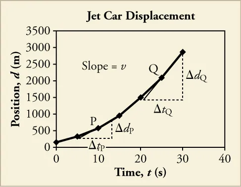
A position–time curve is shown with tangent lines drawn at specific points. The slope of each tangent line represents the instantaneous velocity at that moment, illustrating how “moment-based” velocity is extracted from a graph. This supports the idea that as the time interval shrinks, a secant-slope average velocity approaches the tangent-slope instantaneous velocity. Source

This is the practical bridge between “moment” quantities and measurements you can actually take.

How “Very Small Time Interval” Works in Practice

Approximating instantaneous velocity

To approximate the instantaneous velocity at time $t$, choose two times close to $t$ (one just before and one just after, if possible) and compute $v_\text{avg}=\Delta x/\Delta t$ over that short interval.

The smaller the interval:

• the closer the computed average is to the instantaneous value

• the more sensitive your result becomes to measurement noise

When using position data from a ticker timer, motion sensor, or video analysis:

• keep units consistent (m and s)

• use consistent sign conventions (right/left or forward/backward)

• report an appropriate number of significant figures based on the measurement precision

Approximating instantaneous acceleration

To approximate instantaneous acceleration at time $t$, use velocity values close to $t$ and compute $a_\text{avg}=\Delta v/\Delta t$ over a short interval. This is often done by:

• first determining velocities over small intervals from position data, then

• using nearby velocity values to estimate acceleration over an even smaller interval

Because acceleration is based on changes in velocity, it is typically more sensitive to experimental scatter than velocity. Reducing $\Delta t$ improves the “instantaneous” approximation but can also amplify random error.

Common Interpretation Pitfalls (and How to Avoid Them)

• Confusing average speed with average velocity: speed ignores direction; velocity includes sign.

• Assuming average equals instantaneous: they only match reliably when $\Delta t$ is very small or when velocity/acceleration is constant.

• Using a long interval near a turnaround: if the object reverses direction within the interval, $v_\text{avg}$ may be near zero even though instantaneous speeds were large.

• Mixing intervals: ensure the $\Delta t$ used for $\Delta x$ or $\Delta v$ matches the same endpoints.