
AP Syllabus focus: ‘For constant acceleration in one dimension, three kinematic equations can describe instantaneous linear motion.’
Constant-acceleration kinematics links position, velocity, acceleration, and time for straight-line motion. These three equations let you predict motion at any instant, as long as acceleration stays constant and you define a clear sign convention.
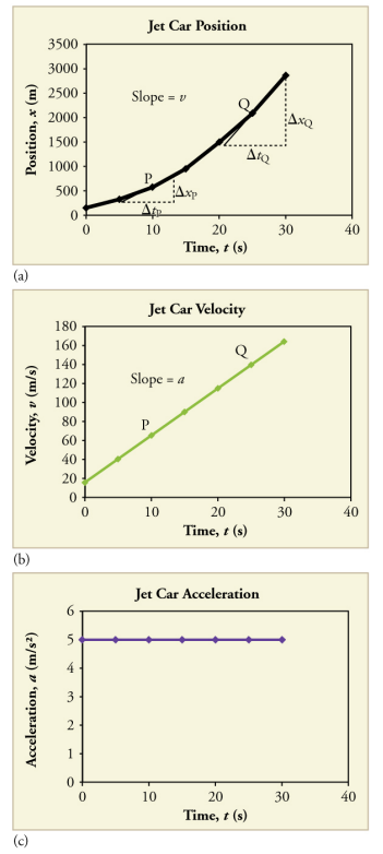
Motion with constant acceleration produces a parabolic position–time curve, a linear velocity–time graph, and a constant acceleration–time graph. The figure highlights that the slope of the vs. curve gives instantaneous velocity, while the slope of the vs. line gives the acceleration. Source
When the constant-acceleration equations apply
The three kinematic equations are valid only for one-dimensional motion with constant acceleration over the time interval of interest. “One-dimensional” means all motion is along a single axis (often called the x-axis), where directions are handled by positive and negative signs.
Constant acceleration — acceleration that does not change with time (both magnitude and direction are constant), so the same value of a applies throughout the interval.
Before using any equation, choose:
A coordinate axis (positive direction).
An origin for position (where x = 0).
A start time (often t = 0), defining initial values.
Variables and initial conditions
You will typically track:
x: position at time t
x0: position at t = 0
v: velocity at time t
v0: velocity at t = 0
a: constant acceleration
t: elapsed time
Displacement — the change in position, equal to final position minus initial position (direction matters).
In 1D, displacement is often written as Δx, and it can be positive, negative, or zero depending on direction and net change in position.
Equation 1: velocity as a function of time
This equation updates velocity when acceleration is constant.
= velocity at time (m/s)
= initial velocity at (m/s)
= constant acceleration (m/s)
= elapsed time (s)
Use this equation when you need velocity after a time interval, or when you need time given a change in velocity. Sign matters: a negative a reduces v if the object is moving in the positive direction.
Equation 2: position as a function of time
This equation connects where the object is after time t, given initial position and initial velocity.
= position at time (m)
= initial position at (m)
= initial velocity (m/s)
= constant acceleration (m/s)
= elapsed time (s)
This equation is especially useful when velocity at the end is not given. The squared time term means that acceleration effects grow more important over longer intervals.
Using displacement form
Sometimes it is cleaner to work with displacement instead of absolute positions. You can treat (x − x0) as displacement Δx in your algebra, but keep the sign convention consistent with your axis choice.
Equation 3: velocity as a function of position (eliminates time)
This equation relates velocities and displacement without using time explicitly.
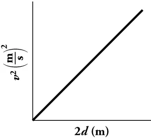
A plot of versus is linear when acceleration is constant, and the slope of the line corresponds to the acceleration. This provides a graphical way to interpret (and experimentally verify) the relationship without using time. Source
= velocity at final position (m/s)
= velocity at initial position (m/s)
= constant acceleration (m/s)
= displacement over the interval (m)
Use this equation when time is unknown or irrelevant (for example, when an object speeds up or slows down over a known distance). Because v is squared, solving for v can produce two mathematical signs; the physically correct sign must match the object’s direction of motion at that moment.
Strategy and common algebra checks
Choosing the right equation
Match what you know to what you need:
If you have a and t, and want v: use the velocity–time equation.
If you have a and t, and want x (or displacement): use the position–time equation.
If you have a and displacement, and want v (no t): use the velocity–position equation.
Consistency checks (high-value habits)
Units: m, s, m/s, m/s^2 must be consistent throughout.
Signs: negative values typically indicate motion or acceleration in the negative axis direction.
Reasonableness: with a = 0, the equations reduce to constant-velocity motion (v = v0, x = x0 + v0 t).
Interval definition: x0 and v0 must correspond to the same start time for the interval you are analysing.
Practice Questions
Q1 (2 marks) A cart moves in a straight line with constant acceleration . Its initial velocity is . Find its velocity after .
Uses (1)
(1)
Q2 (5 marks) A cyclist travels along the x-axis. At , and . The cyclist accelerates at a constant rate for .
(a) Determine the cyclist’s position at .
(b) Determine the cyclist’s velocity at .
(a)
Uses (1)
Substitution of values (1)
(1)
(b)
Uses (1)
(1)
FAQ
They assume a single constant value of $a$ across the whole interval, which is what allows the $t^2$ dependence and the elimination of time in $v^2 = v_0^2 + 2a\Delta x$.
If $a$ varies, you must split the motion into intervals with constant $a$, or use calculus-based methods.
Take $v = \pm\sqrt{v_0^2 + 2a\Delta x}$, then select the sign that matches the direction at that instant.
Use context: if the object is still moving in the positive direction, choose $+v$; if it has reversed direction, choose $-v$.
Yes, provided the acceleration remains constant and you interpret signs correctly.
However, you must be careful: quantities like $\Delta x$ may be small even when the object travels far, and the final velocity sign must match the actual direction at the final time.
Treating $\frac{1}{2}at^2$ as always “adding distance.” It can be negative if $a$ is negative, which correctly represents acceleration pointing in the negative direction.
Also, mixing a positive $v_0$ with a negative direction description is a frequent cause of errors.
Look for internal consistency:
If $a$ and $v_0$ have the same sign, speed should increase over time.
If $a$ opposes $v_0$, speed should decrease and may reach zero at $t = \frac{-v_0}{a}$ (if $a$ is constant and opposite in sign).
Then confirm the sign of $x - x_0$ matches the expected net motion.
