Position-Time Graphs and Instantaneous Velocity (1.3.4) | AP Physics 1: Algebra Notes

AP Syllabus focus: ‘Instantaneous velocity is the rate of change of position and equals the slope of a tangent line on a position-time graph.’

Position–time graphs are a central way to visualise one-dimensional motion. They show how an object’s position changes with time, and they let you interpret direction and changing speed by analysing slope.

Position–time graphs: what you’re looking at

A position–time graph plots position (vertical axis) versus time (horizontal axis). Each point represents where the object is at a particular time.

Higher on the graph means a more positive position (relative to the chosen origin).
A flat (horizontal) segment means position is constant: the object is at rest.
A straight slanted line means position changes at a constant rate: constant velocity.
A curved line means the rate of change of position is changing: velocity is changing.

Reading direction from the graph

The sign of the slope tells you direction of motion in the chosen coordinate system.

Positive slope: motion in the positive direction.
Negative slope: motion in the negative direction.
Zero slope: no motion.

Instantaneous velocity and the tangent idea

Instantaneous velocity comes from the slope at a single instant, not over a long interval. On a position–time graph, that means using a tangent line at the time of interest.

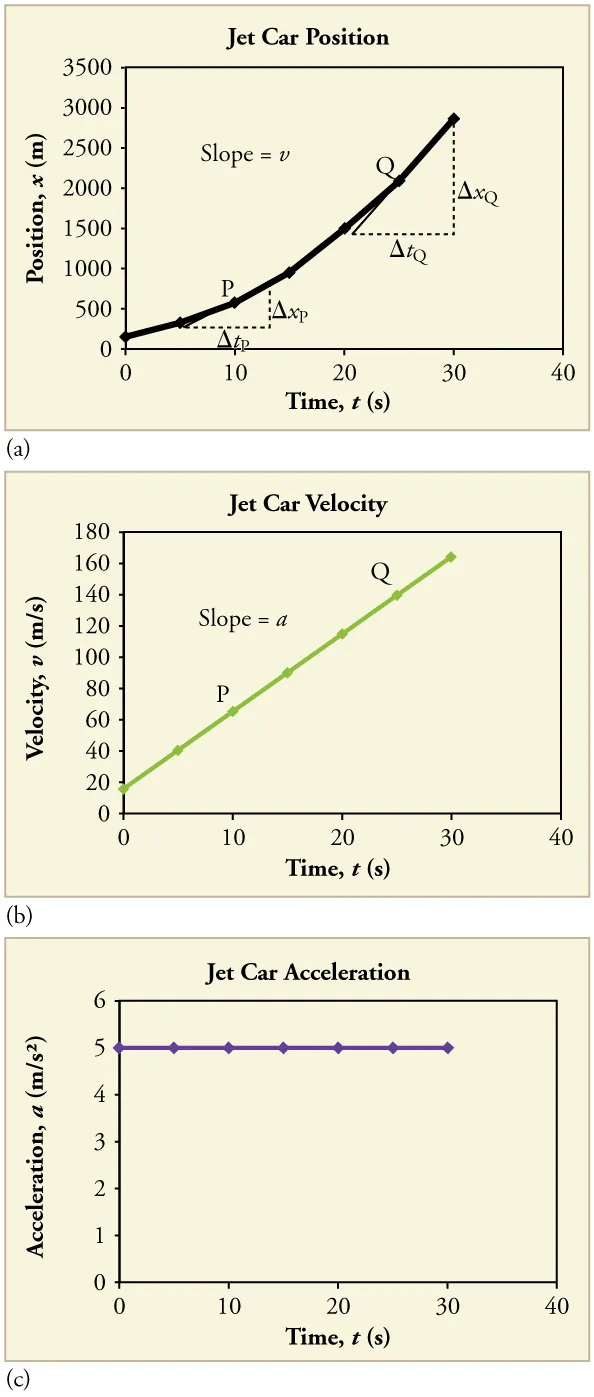
These kinematics graphs illustrate how velocity is extracted from a position–time curve by drawing a tangent line at the instant of interest. The steeper the tangent slope, the larger the instantaneous velocity magnitude, and the sign of the slope indicates direction. This visual also highlights that a curved $x$ – $t$ graph implies changing velocity over time. Source

Instantaneous velocity: The velocity at a specific moment in time; on a position–time graph it equals the slope of the tangent line at that time.

A tangent line is the straight line that just “touches” the curve at one point and has the same local steepness there. For a straight-line position–time graph segment, the tangent line is the line itself, so the instantaneous velocity is the same at every point on that segment.

Slope as a rate of change (what you actually compute)

On a graph, slope is “rise over run”: change in vertical value divided by change in horizontal value.

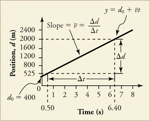
This position–time graph shows a straight line (constant velocity) with the rise and run explicitly marked, reinforcing that slope equals $\Delta x/\Delta t$ . Because the line is straight, the slope is the same everywhere, so the instantaneous velocity matches the average velocity on that interval. The labeled axes also make the velocity units (m/s) immediate from the graph. Source

Here, that is change in position divided by change in time.

$v(t)=\frac{dx}{dt}$

$v(t)$ = instantaneous velocity at time $t$ , in $\mathrm{m/s}$

$x$ = position, in $\mathrm{m}$

$t$ = time, in $\mathrm{s}$

In AP Physics 1 Algebra, you typically estimate the tangent slope by choosing two convenient points on the tangent line (not necessarily on the curve) and computing slope from those coordinates.

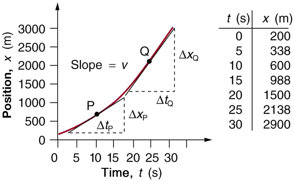
A curved position–time graph is shown with tangent lines drawn at two instants, emphasizing that instantaneous velocity is the tangent slope at the chosen time. The labeled points and read-off coordinates demonstrate the practical “two-point slope” approach for estimating $v(t)$ from a tangent line. This is the graphical meaning of $v(t)=\frac{dx}{dt}$ without requiring calculus to execute the measurement. Source

Estimating instantaneous velocity from a curved graph

When the graph is curved, the slope changes with time, so you approximate the tangent slope carefully:

Identify the time where you want the instantaneous velocity.
Sketch (or imagine) the tangent line at that point so it matches the curve’s local direction.
Pick two well-separated points on that tangent line (to reduce reading error).
Compute slope using those two points: slope equals the instantaneous velocity at that time.

Interpreting magnitude: steepness means speed

The magnitude of instantaneous velocity corresponds to how steep the position–time graph is at that instant.

Steeper tangent → larger magnitude of velocity → larger speed at that moment.
Less steep tangent → smaller magnitude of velocity.
Tangent slope near zero → moving slowly (or momentarily stopped).

Be careful to separate sign (direction) from magnitude (how fast): a steep negative slope means fast motion in the negative direction.

Units and common graph-reading pitfalls

Slope units come directly from the axes:

Position in meters and time in seconds gives velocity in m/s.

Common mistakes to avoid:

Using a secant line across a large time interval when asked for instantaneous velocity.
Computing slope with points on the curve rather than points on the tangent (for a curved graph).
Ignoring the axis scales (non-1 increments can make steepness look misleading).
Confusing “high position” with “high velocity”: velocity depends on slope, not on the position value.

FAQ

A tangent captures the graph’s local steepness at one moment, while a line between two points gives an average over a time interval. If the graph is curved, the slope is changing, so averages can differ substantially from the instantaneous value.

Draw a best-fit tangent that matches the curve’s direction at the point. Then:

choose two far-apart points on your tangent
use large, readable triangles This reduces the percentage error from reading the axes.

At a corner, the slope changes abruptly, so there isn’t a single unique tangent line. In that idealised case, instantaneous velocity at the corner is not well-defined; you can discuss left-hand and right-hand slopes instead.

Shifting the origin changes position values but not slopes, so it does not change velocity. Flipping the positive direction multiplies position by $-1$, which flips the slope sign, so velocity changes sign accordingly.

The physical velocity is unchanged, but steepness can look different if the axes are stretched. Always compute slope using the numerical scales on the axes; do not rely on how “steep” the line appears by eye alone.

Practice Questions

(2 marks) A position–time graph is a straight line passing through $(t=0\ \mathrm{s},, x=2\ \mathrm{m})$ and $(t=4\ \mathrm{s},, x=10\ \mathrm{m})$ . Determine the instantaneous velocity.

Uses slope idea for instantaneous velocity on a straight line: $v=\Delta x/\Delta t$ (1)
$v=(10-2)/(4-0)=2\ \mathrm{m,s^{-1}}$ (1)

(5 marks) A position–time graph is curved. At $t=3.0\ \mathrm{s}$ , a tangent is drawn. Two points on the tangent are $(2.0\ \mathrm{s},, 5.0\ \mathrm{m})$ and $(4.0\ \mathrm{s},, 1.0\ \mathrm{m})$ . a) Determine the instantaneous velocity at $t=3.0\ \mathrm{s}$ . (2) b) State what the sign of your answer indicates about the motion at that time. (1) c) Without further calculation, explain whether the speed at $t=3.0\ \mathrm{s}$ is greater than, less than, or equal to $1\ \mathrm{m,s^{-1}}$ . (2)

a) Correct method: $v=\Delta x/\Delta t$ using tangent points (1)
a) $v=(1.0-5.0)/(4.0-2.0)=-2.0\ \mathrm{m,s^{-1}}$ (1)
b) Negative velocity indicates motion in the negative direction (1)
c) Recognises speed is magnitude of velocity, $|v|=2.0$ (1)
c) Compares $2.0>1.0$ , so speed is greater than $1\ \mathrm{m,s^{-1}}$ (1)

Try All Topic Practice Questions

Written by:

Dr Shubhi Khandelwal

Qualified Dentist and Expert Science Educator

Shubhi is a seasoned educational specialist with a sharp focus on IB, A-level, GCSE, AP, and MCAT sciences. With 6+ years of expertise, she excels in advanced curriculum guidance and creating precise educational resources, ensuring expert instruction and deep student comprehension of complex science concepts.