When you describe a quantitative distribution, you translate a graph into statistical language. A complete description explains the overall pattern, where typical values lie, how much the values vary, and whether anything stands out.

Describing a Quantitative Distribution

In AP Statistics, a distribution is usually described from a histogram, dotplot, or stemplot. The goal is not to list every data value. Instead, identify the most important visual features and explain them in context of the variable being measured.

A useful description tells a reader what the data look like without showing the graph. For one-variable quantitative data, focus on four ideas: shape, center, spread, and unusual features.

Shape

Shape refers to the overall form of the distribution. Ask where most observations are, how the tails behave, and how many prominent peaks appear.

A distribution may be roughly symmetric, meaning the left and right sides look similar.

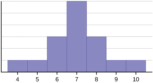
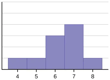
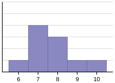
Three contrasting histograms illustrate a symmetric distribution and two skewed distributions (left-skewed and right-skewed). The side with the longer tail identifies the direction of skew, which is the core visual cue students should translate into words when describing shape. Seeing the three shapes side-by-side makes it easier to connect “overall form” and “tail behavior” to precise statistical language. Source

It may be skewed right, with a longer tail on the high-value side, or skewed left, with a longer tail on the low-value side. Shape also includes modality: some distributions have one clear peak, while others have two or more distinct peaks.

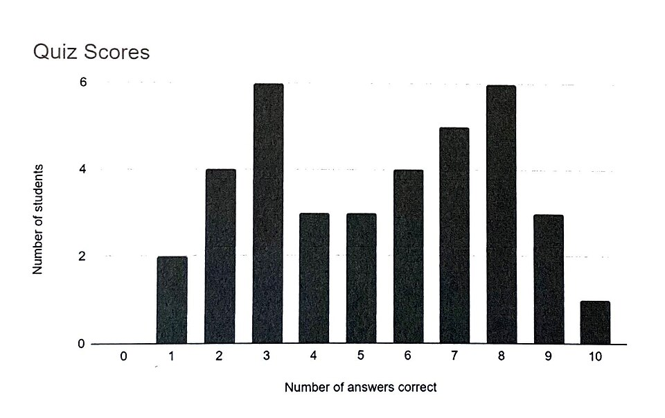
A bimodal distribution is shown with two distinct peaks separated by a lower-density “valley.” This is a canonical example of why a single measure of center can be misleading: the mean or median may fall near the valley even though relatively few observations occur there. The figure supports careful description of shape by explicitly highlighting multiple peaks as part of the overall pattern. Source

In some cases, bars or dots are spread fairly evenly across values, giving an approximately uniform appearance.

When describing shape, use cautious language such as approximately, appears, or roughly. Real data are rarely perfectly symmetric or perfectly uniform.

Center

Center is the location of a typical observation. On a graph, it is often estimated rather than read exactly. For example, you might say that the distribution is centered around 52 minutes or that a typical score is in the mid-70s.

The center should match the shape of the data. If the distribution is fairly symmetric, the mean and median are often close, so either idea of center may represent the data well. If the distribution is strongly skewed, the median is often a better description of a typical value because extreme values can pull the mean toward a tail. Even when you do not calculate a statistic, you should still identify the general location of the center.

Spread

Spread describes how much the observations vary. A distribution with little spread has values packed closely together. A distribution with large spread has values scattered over a wider interval. Two data sets can have the same center but very different spread, so both features matter.

On graphs, spread is usually described with words and approximate intervals. You might note that values run from about 10 to about 90, or that most observations fall between 30 and 45. Spread helps answer whether the data are consistent or highly variable. When writing in context, describe spread using the variable's units, since a spread of 5 could mean very different things for test scores, ages, or reaction times.

Unusual Features

After describing the general pattern, look for values or regions that do not fit the rest of the distribution. These are unusual features.

An outlier may suggest an error, but it may also be a real and important observation. Do not automatically remove it or assume it is wrong; simply note that it is separated from the main body of data.

Other unusual features include gaps, clusters, and multiple peaks. A gap is an interval with no observations. A cluster is a region where many observations are grouped closely together. Multiple peaks can indicate that the data may come from different subgroups or that more than one common value exists. These features matter because they can hide behind simple summaries. For example, a single center may not describe a bimodal distribution very well, and a wide spread may actually reflect two separate clusters rather than one broad pattern.

Writing a Strong Description

A complete AP Statistics description should be specific, concise, and connected to the context.

• Identify the variable and its units.

• Describe the shape using terms like symmetric, skewed, unimodal, or bimodal.

• Give an approximate center.

• Comment on the spread using an interval or a general statement about variability.

• Mention any unusual features, such as outliers, gaps, clusters, or multiple peaks.

• Use contextual language, such as "student study times" or "daily temperatures," not just "the data."

Good descriptions combine several features in one sentence or short paragraph. Instead of saying only that a graph is skewed, explain where it is centered, how wide it is, and what stands out. That fuller description is what makes statistical communication useful.