In this section, you learn how a chosen confidence level leads to a specific critical value, linking probability ideas to practical confidence interval construction methods.

Determining the Critical Value

When constructing a confidence interval for a population proportion, the critical value is the specific multiplier that stretches the margin of error to match your chosen confidence level. It connects the desired reliability of the interval to the variability described by the standard normal distribution.

Because the critical value comes from a probability model rather than your particular dataset, it depends only on the confidence level and the assumption of an approximately normal sampling distribution, not on the sample itself.

When you select a confidence level, you are choosing what proportion of intervals, in repeated sampling, you want to capture the true population proportion.

The higher the confidence level you demand, the larger the critical value must be, which in turn makes the interval wider.

The Standard Normal Distribution and z-Scores

To determine the critical value, AP Statistics uses the standard normal distribution, a bell-shaped curve with mean 0 and standard deviation 1, measured in z-scores.

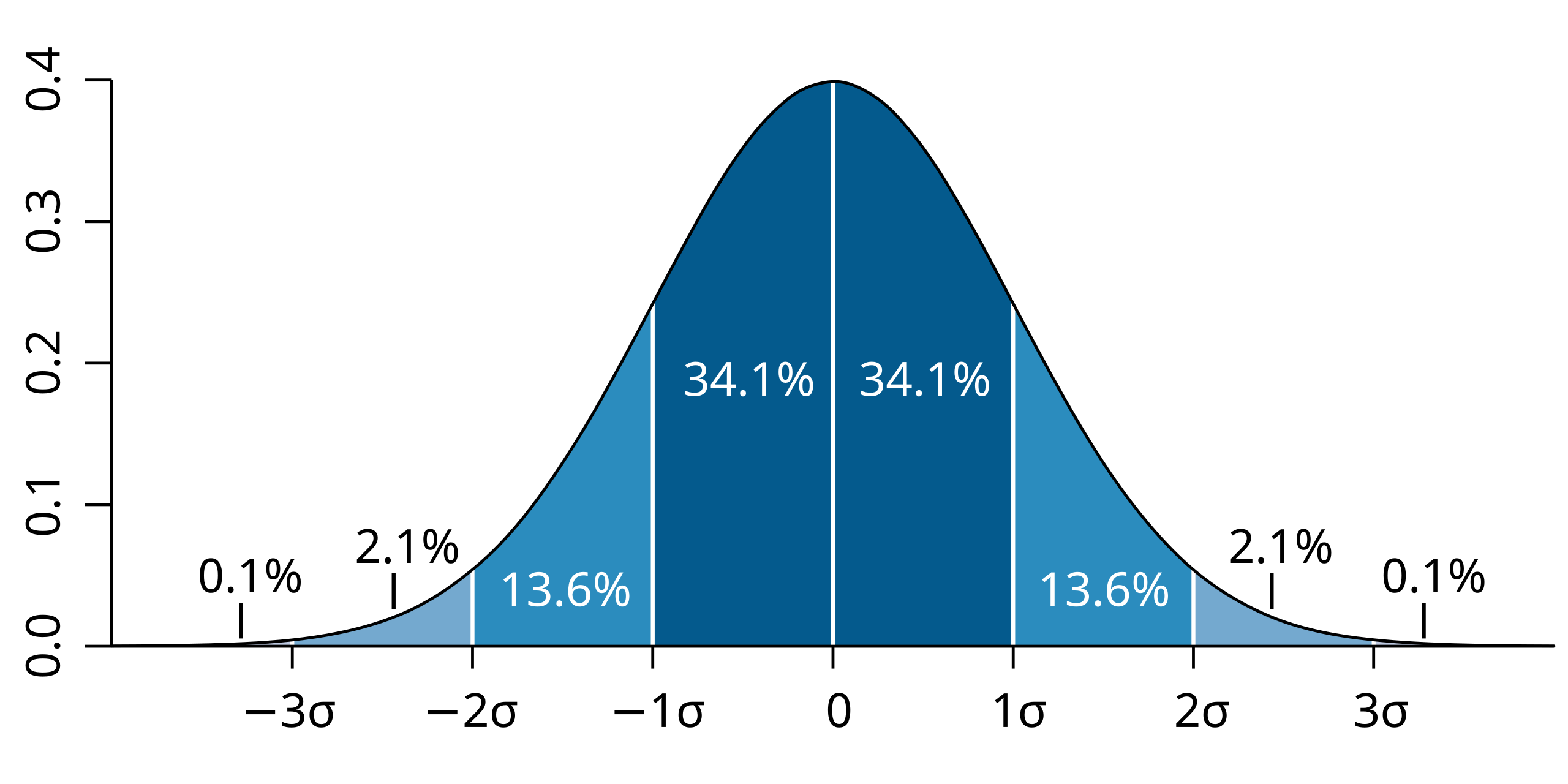
A standard normal distribution centered at 0, with each standard deviation highlighted and labeled. The shaded percentages show how much area falls within 1, 2, and 3 standard deviations of the mean. The additional numerical labels exceed the strict syllabus requirements but help illustrate how z-scores correspond to probability. Source.

A z-score tells you how many standard deviations an observation is above or below the mean. For confidence intervals, the critical value z* is a z-score that cuts off the appropriate central area under this curve.

The standard normal distribution is symmetric about 0, so the central area between −z* and +z* equals the chosen confidence level, while the remaining area is split equally between the two tails.

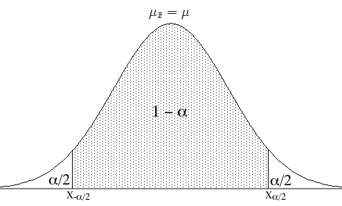
A normal curve with the central probability region shaded and the endpoints labeled by the critical values. The diagram shows how confidence levels correspond to central areas and tail probabilities. The α and z_{α/2} notation slightly extends beyond the syllabus wording but matches AP Statistics conventions. Source.

Linking Confidence Level to the Critical Value

To find the critical value for a particular confidence level:

• The central area between −z* and +z* should equal the confidence level (for example, 0.95 for 95% confidence).

• The tail area outside the interval is 1 − confidence level.

• Because of symmetry, each tail has area (1 − confidence level) ÷ 2.

This relationship allows you to map confidence levels to standard critical values.

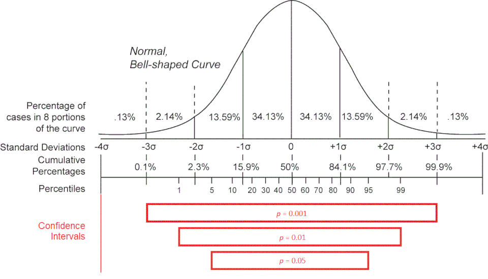
A sequence of normal curves displaying central intervals of various widths, each corresponding to a different confidence level. Wider intervals represent higher confidence levels and larger critical values. Some probability labels use p-notation not explicitly required by the syllabus but consistent with general interval theory. Source.

Common examples for two-sided confidence intervals for a proportion include:

• 90% confidence: z* is approximately 1.645

• 95% confidence: z* is approximately 1.96

• 99% confidence: z* is approximately 2.575

These values come from standard normal tables or technology and are treated as known constants at the AP level.

Practical Procedure for Determining z*

In practice, determining the critical value involves a consistent set of steps:

• Specify the confidence level (for example, 90%, 95%, or 99%) based on the context of the problem and how much certainty is desired.

• Convert the confidence level to a central probability between −z* and +z* on the standard normal curve.

• Compute the tail area as 1 minus the central probability, then divide by 2 to find the area in each tail.

• Use a z-table or technology (such as a calculator’s inverse normal function) to find the z-score with cumulative area equal to the left-tail probability.

• Take the positive z-score as the critical value z* for the two-sided confidence interval.

Because the distribution is symmetric, you only need the positive z* when constructing intervals; the negative counterpart simply marks the lower bound on the other side of the mean.

Using the Critical Value in Margin of Error and Confidence Intervals

Once you know z*, you can use it to determine the margin of error and then the full confidence interval for a population proportion. The margin of error is the product of the critical value and the standard error of the sample proportion.

EQUATION

Here, z* directly controls how far the interval extends from the sample proportion. A larger z* produces a larger margin of error and therefore a wider interval, while a smaller z* produces a narrower interval.

Choosing an Appropriate Confidence Level (and Thus z*)

Selecting a confidence level is a modeling decision that determines the critical value you will use. Important considerations include:

• Required certainty: Situations with serious consequences for incorrect conclusions often justify higher confidence levels, which produce larger z* values.

• Desired precision: Higher confidence (larger z*) increases interval width, reducing precision. Lower confidence narrows the interval but reduces the long-run capture rate of the true parameter.

• Feasibility of larger samples: If the sample size cannot be increased, the only way to reduce interval width is to choose a lower confidence level, which corresponds to a smaller z*.

In every case, determining the critical value means translating the verbal demand for a certain level of confidence into a precise numerical multiplier taken from the standard normal distribution, ready to be used in the margin of error and confidence interval formulas.