Constructing a confidence interval for a population proportion provides a structured method to estimate an unknown population value using sample data, combining point estimates with measures of sampling uncertainty.

Constructing a Confidence Interval for a Population Proportion

Constructing a confidence interval for a population proportion involves combining three essential components: the point estimate, the critical value, and the standard error to produce a range of plausible values for the true population proportion. This process aligns directly with the syllabus requirement to apply the formula $\hat{p} \pm z^*\sqrt{\frac{\hat{p}(1-\hat{p})}{n}}$ and emphasizes the conceptual meaning behind each part of the interval.

Understanding the Components of the Confidence Interval

The confidence interval is built on the sample proportion $\hat{p}$, which serves as the best estimate of the population proportion. To account for sampling variability, the construction incorporates a margin of error, combining the variability measure (standard error) with the confidence-level–dependent critical value.

Using the point estimate alone is insufficient because sample data naturally vary from sample to sample. Therefore, constructing the entire interval provides a fuller picture of uncertainty in the estimate.

Identifying What the Formula Represents

The confidence interval formula uses the standard error of $\hat{p}$ to quantify expected sampling variability and the critical value to scale that variability according to the chosen confidence level.

EQUATION

This formulation integrates all major ideas required for constructing the interval: the central estimate, its variability, and the multiplier that adjusts for the desired level of confidence.

A critical sentence explaining these components connects the formula to the logic of statistical inference.

Steps for Constructing the Confidence Interval

To ensure clarity and accuracy, constructing a confidence interval for a population proportion typically follows a structured sequence. Each step relies on the previous one, reinforcing the importance of conceptual understanding and procedural correctness.

Follow this process:

• Identify the point estimate ($\hat{p}$).

  • Compute using the number of successes divided by the sample size.

• Check that conditions are met.

  • Independence and normality conditions must be verified before using the interval formula, though these checks are addressed in earlier subsubtopics.

• Calculate the standard error using the formula $\sqrt{\frac{\hat{p}(1-\hat{p})}{n}}$.

• Determine the critical value ($z^*$).

  • This corresponds to the chosen confidence level (e.g., 1.96 for 95%).

• Compute the margin of error by multiplying $z^*$ and the standard error.

• Construct the confidence interval using $\hat{p} \pm \text{margin of error}$.

• Interpret the interval in context, focusing on what the range suggests about the population proportion.

Written in words, a confidence interval has the form point estimate ± margin of error.

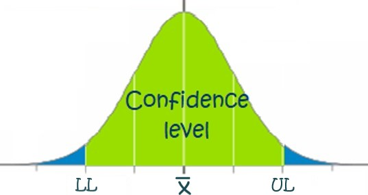
A visual representation of a confidence interval on a normal curve, with LL and UL marking the lower and upper bounds. The shaded region represents all plausible values for the parameter at the chosen confidence level, while the tails show unlikely values. Although generic, the structure directly parallels the one-sample z-interval for a population proportion. Source.

The Role of Each Component

Each part of the confidence interval formula contributes uniquely to understanding the likely location of the population proportion:

• The point estimate anchors the interval in observed data.

• The standard error expresses sampling variability, becoming smaller as sample size increases.

• The critical value expands or contracts the interval depending on the desired confidence level.

• The margin of error combines standard error and critical value to reflect the total uncertainty.

This explanation clarifies how the interval balances the precision of the estimate with the uncertainty inherent in sampling.

The critical value z* comes from the standard normal distribution and cuts off the middle C% of the area, leaving α/2 in each tail.

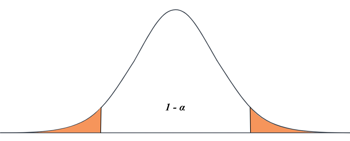
A standard normal curve showing how the critical values ±z* define the middle (1−α)100% of the distribution. The shaded region represents the confidence level, while the unshaded tails represent the remaining α. This geometry underlies the selection of z* for the one-sample z-interval for a population proportion. Source.

Why Constructing the Interval Matters

Constructing a confidence interval allows statisticians to express uncertainty using a quantitative range rather than a single point estimate. The interval communicates both the sample result and the degree of confidence that the method will capture the true population proportion in repeated sampling.

The procedure is valuable because:

• It provides an interpretable range for the unknown population parameter.

• It accounts for the variability expected in different random samples.

• It incorporates the analyst’s chosen confidence level, reflecting how cautious they wish to be.

Bringing the Components Together

The constructed interval presents a balance of empirical evidence and theoretical justification. By integrating the components—point estimate, margin of error, and critical value—the method produces an interval that quantifies uncertainty and frames inference in terms of probability and sampling behavior.